Neural Networks and the Backpropagation Algorithm

March 23, 2015

The other day I had been looking up information on machine learning. I’m new to some of the topics in this field but I have been introduced to them before. I’ve always wanted to learn more. The idea of teaching a computer how to “learn” just seems intriguing to me.

Specifically I had been researching neural networks. They are useful because they can help uncover hidden patterns in a plethora of data, or be taught to perform certain tasks such as handwriting or facial recognition.

I had watched an MIT OpenCourseWare Lecture which gave a rough introduction to neural networks which I found to be quite captivating. I found it so fantastic actually that I wanted to share the basic concepts here. For the purpose of this post, I’m going to assume that we’re teaching this neural net via supervised learning.

In other words, we are going to make this neural network learn by giving it a set of “correct” input and output values, which it will use to calibrate, or change its own structure to make sure that it also outputs the correct values. Let’s dive in!

To explain briefly, neural networks are modeled after the same neurons that exist in our brain.

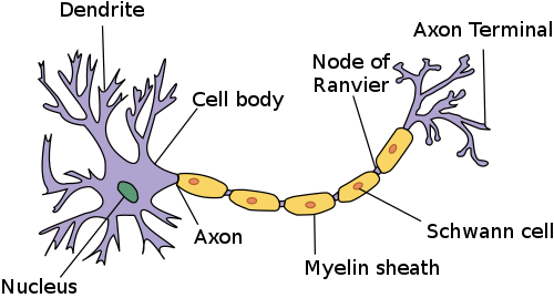
For our purpose we are going to focus on only a few of the main features of a neuron which are critical to the model of neuron.

The main parts that we are going to focus on:

• Dendrites
• The Axon
• The Axon Terminals

The dendrites are small tree-like structures that are stimulated when enough neurotransmitters are dumped into the synapse between a neuron and the end of the dendrite. Some of these dendrites might be easier to stimulate than other based on various factors

The axon is the lengthy part of the neuron which simply propagates a “spike” of energy to the axon terminals, which originates from the dendrites.

The axon terminals dump neurotransmitters into the synapse to help stimulate the dendrites of the next neuron.

At the end of each axon terminal there exists another neuron’s dendrites separated by a tiny gap of space called the synapse. When a neuron is stimulated, it will dump neurotransmitters into the synapse. If there are enough neurotransmitters dumped into the synapse, It will stimulate the next neuron’s dendrites, sending a spike of “excitement” or “energy” to the next neuron, and so forth.

You can imagine some synapses being smaller or larger, needing more or less neurotransmitters to excite a neuron.

This is a gross simplification of a neuron, but for the model of a neural network, we don’t need to understand more than this.

Modeling the Neuron

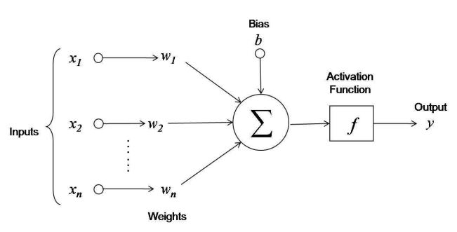
First, notice the inputs. Each input from \(x_1\) to \(x_n\) is given as an input to the neuron. Each of the inputs is multiplied by a weight \(w\) corresponding to an input before being summed into the function.

The neuron also has a bias, labeled \(b\) in the diagram, which I like to call \(w_0\). We can think of this bias as a given input to each neuron that always has a value of -1. The weight of the bias input \(w_0\) can be adjusted accordingly.

Think of each input multiplied by a weight representing a neurotransmitter that is dumped into a synapse between neurons by one of the axon terminals.

From here we can represent the total stimulus as the sum of each input multiplied by a corresponding weight.

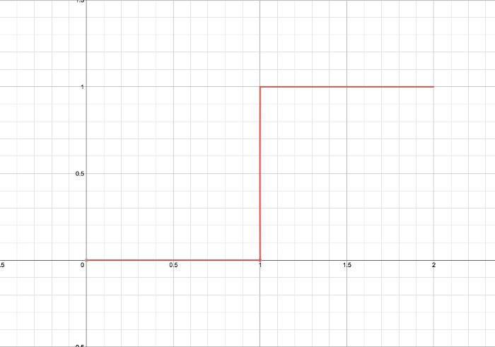
The value of this will be then be passed onto the activation, or threshold function. The threshold function might be best viewed as a single-step function, where say once the input \(\alpha\) reaches a certain value, it will output a certain value. We’re going to keep this to ones and zeros.

This part is where the dendrites need to pick up enough neurotransmitter signals to send that spike of “energy” or “excitement” down its axon to the axon terminals.

Next, once the threshold is activated or not, we will get an output from this neuron. We can string many neurons together and in different patterns with different layers to create a network. More complex networks take up more computational power, but they can also convey more complex functions.

Once we create and run a test using our own neural network, we are going to need to find out how good (or bad) the neural network did at calculating our answer.

Remember how I said that the neural network is given a set of “correct” inputs and outputs to learn from? Well here’s where that comes into play.

Let’s say that our output of the neural net is \(z\) and our desired or correct output is going to be assigned to \(d\). We are going to need a function to test our performance of the neural network.

Let’s call this function \(P\). Also, for simplicity’s sake, and because this is convenient we’re going to make the performance function the following:

(You’ll see what I mean by convenient later)

Adjusting the Model

So now we’ve got this model. We have a function to test whether our output is close to what we want it to be. We have a way to add our inputs together. What comes next?

Well, we need to have some way of adjusting the neuron to make sure we get closer to our desired output. But how do we know what to adjust? and by how much?

We’re going to use a method called gradient descent (or ascent depending on direction). This will help us determine which direction we need to move our weights in to get closer to the desired value, \(d\). Be prepared for lots of math.

So we know that our desired outputs \(d\) can be given by \(\overline{d} = g(\overline{x})\); where \(\overline{d}\) and \(\overline{x}\) are our vectors of inputs and desired outputs that our neural network is going to learn from.

The problem is that we don’t know what function \(g\) is, which is why we’re using the neural network to represent it. With the neural networks, we can represent our inputs and outputs by a multivariate function \(f\). This function can be represented by \(\overline{y} = f(\overline{x}, \overline{w})\).

Given these functions, we can see our performance function is now

We can see from here the performance function is really just a function of the inputs, \(x\) and the weights \(w\).

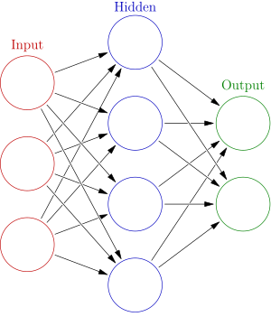
Now imagine that we add some complexity to our neural network. We are going to chain together multiple neurons to create layers. We can then chain these layers together. The more chains and connections between neurons the more complex are the things we can model or predict.

Mathematically speaking for this network we have vectors \(\overline{x}\) and \(\overline{w}\) for each layer. The individual values of \(\overline{w}\) are the values we modify in our network to conform the inputs to the desired outputs.

Just imagine the above diagram of the neural network laid end to end and on top of each other. A general overview can be seen below, where each circle represents a neuron:

This is where things start to become more interesting. Using the algorithm of gradient descent, we can alter the weights \(\overline{w}\) by taking the gradient of our performance function with respect to each weight. We can also multiply this gradient by a rate constant, let’s say \(\delta\), that will determine how much we alter the weights over each iteration.

So let’s look at our formula

This is now telling us that the change in our \(w\) over each iteration is going to be equal to \(\delta\) multiplied by the partial derivative of \(P\) with respect to each weight.

But wait! We have a problem here. We can’t just simply take the partial derivative of \(w\) with respect to \(P\) because \(w\) lies within our other function \(f\). This means that we are going to need the chain rule.

So this brings up another problem: because we are going to need to take all these derivatives all of the functions in our neural network must be differentiable.

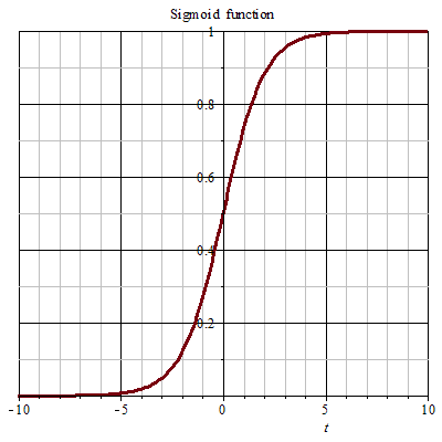
So the problem of differentiability lies within our step function. Because a step function is not differentiable we need another function to replace this. Fortunately there is one similar to it that is differentiable!

It’s called a sigmoid function. You might have seen it before. It has the form

This function also happens to be convenient. (You’ll see why in a second)

The graph of the sigmoid has the following shape:

.

Great! So where do we go from here?

Well, I suggest you watch the video I linked earlier if you want a really good understanding of how this works. I will do my best to explain it, but I won’t go into explicit detail of how this all works together. The video will explain things more thoroughly.

So if we keep taking our partial derivatives with the chain rule, it turns out that we will need to take the derivative of this sigmoid function and the performance function.

The sigmoid function just so happens to be pretty neat. Let’s call it \(\beta\). If you take the derivative of this function and we manipulate it a bit, that the derivative of the sigmoid turns out to be expressed in terms of the original function itself. I’ll let the math do the talking here.

Then we rearrange our derivative a little bit:

Voila! The derivative of the sigmoid function turns out to be given in terms of the original! I find that to be quite astounding. If you don’t believe me you’ll just have to take my word for it. I promise you it works. (This is also why I called this function convenient).

Now lets do the derivative of the performance function, \(P\). We need to take the derivative with respect to the neuron’s output, \(y\).

It’s pretty simple, so I’m not going to go into it, but \(\frac{\partial P}{\partial y} = (d - y)\).

So it turns out to be a pretty simple derivative, which is why this function just so happens to be convenient for our purposes.

Calculating The Change via Backpropagation

Calculating the change for each weight isn’t as simple as a single derivative as the neurons in a hidden layer put a bunch of junk in the way, so we end up needing the chain rule. That math can get pretty messy, so I’m going to do my best to simplify it.

So just as a refresher, let’s look at what we need to calculate. Remember than \(w_0...w_n\) represents just the weights of a single neuron. We have to calculate the adjusted weights for every neuron of each layer in our neural network.

Let’s start by considering the neurons in the very last layer of the network, the output neurons. These require the least amount of work to calculate because we simply need the derivative of the perfomance function, the derivative of the sigmoid.

Consider \(\gamma_{n}\) where n represents an arbitrary number between \(0\) and \(N\) for each neuron. \(y_n\) is the output of the threshold function from the neuron on layer \(L\) where, \(L\) represents the network layer on which variable lies.

\(\gamma_{n}\) will be equal to the following if it is an output neuron. Remember \(z\) is the final output and \(d\) is desired output.

and if gamma is an inner or “hidden layer” neuron

So now that we have \(\gamma_n\), the change in weight for a given neuron on the output layer is

Wrapping Up

So what does all of this mean?

If we take a look at the math, starting at the output neurons, we calculate their \(\gamma_n\) values which rely on the network’s output. We can do this fairly quickly for our output layer.

Then we’ll move another layer closer to the starting point of our network. The change in their weights for the networks depends on the \(\gamma_n\) of the layer in front of it, which we happened to have already calculated.

What this means is that when we are calculating exactly how to adjust the weights in our neural network, the change in each weight depends on a few things.

• The input to the neuron
• The output of the neuron
• The weight of the neurons in the layers closer to the output.

This helps explain why it’s called the backpropagation algorithm. You need to calculate the change in weights at the end of your neural network before you can calculate the change in the beginning. So you work your way back in a wave-like manner, hence the name backpropagation.

The other great thing about this algorithm is that the change in weight depends on things you’ve already calculated, or things you’re going to have to calculate anyways. It’s extremely effecient. There are few, if any, wasted computations.

And that’s simply it. The most basic of neural networks and the backpropagation algorithm.

Credits

This whole post was a learning experience for me, so I feel I should give credit where credit is due.

• MIT Lecture, inspiration for this post
• Wikipedia page on the backpropagation algorithm
• PDF from Caltech
• Wikimedia for some images

For any corrections to this post, please leave a comment.