A (Somewhat) Comprehensive Guide to Physics 227 at Rutgers University
Click here to go back to the Physics 227 page
So here we are again - another semester of introductory physics at Rutgers University, New Brunswick. This is the Fall 2015 semester. This will be a kind-of continuation from the Physics IB guide from the previous spring 2015 semester.
The aim of this is post/page to provide a (somewhat) comprehensive guide to this class by periodically updating it throughout the semester. My plan is to make notes during lecture as well as provide practice problems and explanations.
Without furthur ado - Let’s dive in!
September 3rd, 2015
Almost everything in the universe can be described by just 4 (!) equations.
Electric Charge
- Electric Charge is a physical quantity that characterizes how charged object participate in electrostatic interactions
Electric Charge Properties
- It is a scalar value
- It is quantizes - meaning that a charge must be in integer multiples of the fundamental value of charge
- This fundamental amount is the charge of an electron.
\[e = 1.6 \cdot 10^{-19} Coulombs\]
- The net charge of any isolated system is conserved. i.e the net charge of the universe is zero
Coulomb’s Law
Coulomb’s law describes the forces that charged particles exert on each other due to…well…simply their charge.
The equation for Coulomb’s law is the following:
\[F_{12} = k\frac{\left|q_1q_2\right|}{r^2}\]
Now let’s quickly describe each quantity
- \(F_{12}\) is the force that each particle exerts on one another. This means that both particles experience the same force!
- \(k\) is a constant value expressed in this function. It’s value is equal to \(\frac{1}{4\pi\epsilon_0}\)
- \(q_1\) and \(q_2\) are the charges of each particle measured in Coulomb’s or the symbol \(C\)
- \(r\) is the distance between the two charges.
\[k = \frac{1}{4\pi\epsilon_0} = 9*10^9 \frac{Nm^2}{C^2}\]
\[\epsilon_0 = 9 * 10^{-12} \frac{C^2}{Nm^2}\]
The Superposition Principle
- This principle states that the interaction between any two charges is unaffected by any other charges present
- This principle also tells us that the equations are linear. The solutions of multiple equations can be added together to form other solutions (as in the presence of multiple charges).
Electric Dipole
An electric dipole is formed by two charges \(+q\) and \(-q\) at the distance \(d\) apart.
And that wraps up section one! I hope to keep this as up to date as possible. If you would like to contribute to this guide please submit a pull request on GitHub.
September 6th 2015
Lecture 2 - Electric Field and Electric Field Lines.
One great analogy for electrostatic fields is gravity. Think about it
Gravity is a force we feel due to mass. All around a massive object, the force due to gravity than another object would feel is always directed at the center of mass of the larger object no matter the position around the massive object.
Now think about a negatively charged object with no mass (and every other object is a positively charged object). Every positive object would undergo a force directed at the very center of the negatively charged object (so long as it is a point charge). It wouldn’t matter the location of the positive test charges. The force is always pointing towards the same point on the negatively charged object.
Electric Field
- Units are in \(\frac{N}{C}\)
- A force due to an electric field can be defined as \(\vec{F} = q\vec{E}\)
- Another form: \(\vec{E} = k\frac{q}{r^2}\)
It’s very useful to know that due to the superposition principle (mentioned above) We can add vectors of electric fields to find the net electric field due to multiple charges, simply by adding the fields due do different charges at a single point. To add fields from different charges together, you must be using the same test-point for each field.
Electric Field Lines
- The direction of the electric field vector is tangential to the field line (curve)
- The intensity of the electric field at a given point is proportional to the local density of the field lines.
Another way of stating it, is that at every point on a field line, the force experienced by a test charge is in a direction that is tangential to the field line.
More things to note:
When drawing electric field lines, the lines should always point away from a positive charge, and either terminate at a negative charge, or at infinity.
- A weaker field will have less lines (less dense)
-
A stronger field will have more lines (more dense)
- For a point charge: \(E(r) \propto \frac{1}{r^2}\)
- The density of the lines is \(\propto \frac{1}{r^2}\)
- The area of a sphere centered at the charge is \(\propto r^2\)
Electric Polarization
Redistribution of charges within a neutral object by an external electric field. As a result, a neutral object acquires a dipole moment.
We call materials that have induced or built-in dipoles, dialectrics. For example water. Dialectrics are usually insulators.
If we apply an electric field to any of these dialectrics, they will polarize themselves. As is one side of the object will become more positive, and one more negative.
On the other hand, we have conductors that can polarize themselves because their electrons act as a “sea”. The electrons flow freely inside the metal. So if you apply and electric field, the electrons will move in the directon of the electric field, leaving some parts more positively/negatively charged than others.
September 10th 2015
Lecture 3 Electric Field Flux and Gauss’ Law
Quick review question:
Imagine there is a negative charge, \(-Q\), in an electric field. It is released from rest. What direction will the particle’s acceleration be?
- The particle will travel opposite the direction of the electric field. Positive charges will flow with the field, negative flow in the opposite direction.
Electric Flux
First, imagine water flowing through a pipe. How would you find the flow rate? Most people will probably want to use an equation similar to \(\Delta{V} = A \cdot v \cdot 1s\)
Now what happens if we don’t take a perfect cross section of the pipe though? How can we calculate the flow rate through this new cut? (Imagine the cut being at an angle to the edge of the pipe rather than perpendicular). Turns out we can still find the flow rate even though the cut is different.
All we have to do is simply take a dot product (or multiple through by \(cos(\phi)\)).
-
So the flow rate for a different (non-perpendicular cut) is \(\Delta{V} = \vec{A} \cdot \vec{v} \cdot 1s\) or \(\Delta{V} = Av cos(\phi)\).
-
Equation for flux
\[\Phi_a = \vec{a}(\vec{r}) \cdot d\vec{A} = a(r)A \cdot cos\phi\]
- Units of flux: \(\frac{Nm^2}{C}\)
- Another Form: \(\Phi_E = \vec{E} \cdot \vec{A} = \int\vec{E}(\vec{R}) \cdot d\vec{A}\)
Point Charge at the Center of a Spherical Object
At each point of a surface \(\vec{E} * d\vec{A}\) where \(( cos\phi=1 )\)
Simplified, this means that the flux for a spehere is equal to \(\frac{1}{4\pi\epsilon_0}\frac{q}{r^2}4\pi r^2\)
This expression is equal to \(\frac{q}{\epsilon_0}\)
- So what if we pose the question: What would be the flux of the gravitational field of Earth, through Earth’s surface?
Flux of Graviatational Field \(= -4\pi G M\)
For fields that have \(\frac{1}{r^2}\) dependence, it is true that any field lines entering an object’s surface must also exit. This means that the flix for any surface not contianing any charge, the flux is zero.
This also means any surface deformations do not have an effect on the flux of the object.
- Put simply this means that for any and all objects, the flux is dependent only upon the sum of the charge within the object,
From the lecture notes:
For any closed surface, the flux of the electrostatic field would be proportional to the net charge inside the surface.
- Gauss’ Law is also valid in electrodynamic, not just electrostatics because it is valid for any point inside of an object.
- Gauss’ Law: First of Maxwell’s Equations.
Applications of Gauss’ Law
- Gauss’ Law in its integral form (one scalar equation) is not sufficient for finding three components of a vector field, E.
- However, Gauss’ Law is very useful whenever it is possible to reduce a 3D (vector) problem to a 1D (scalar) problem.
Useful symmetries:
- Sphereical Cylindrical + translational
- Plane
an example of insufficient symmetry could be an electric dipole.
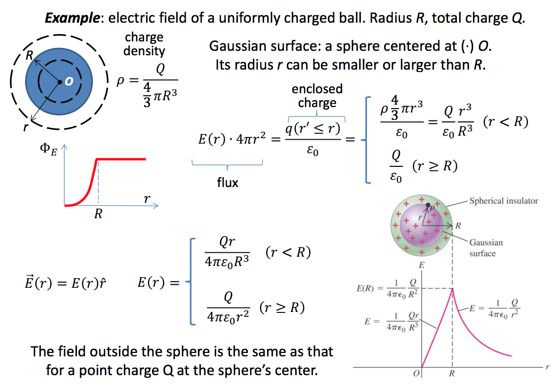
Spherical Symmetry
Ex: The electric field of a uniformly charged ball. Radius \(R\), Total charge \(Q\).
- Gaussian surface: a sphere centered at the origin O. It’s radius \(r\) can be smaller or larger than \(R\).
September 14th 2015
Lecture 4 - Conductors in Electrostatics
The general problem of electrostatics is that given object carry many different charges - and we want to find out the electric field
Reminder: Gauss’ Law
\[\int \vec{E}(\vec{r}) \cdot d\vec{A} = \frac{Q_{net}}{\epsilon_0}\]
Basically the law tells us that the integral over a sphere of an electric field (a vector) dot-multiplied by the differential area will give us the flux - which for any sphere can be simplified to \(\Phi = \frac{Q_{net}}{\epsilon_0}\)
Matter in Electrosatic Fields
Conductors
-
Electrons flow freely inside the metals - they will arrange themselves based on the field applied to the metal
-
An electric field applied to a metal will cause the electric field inside the confuctor to become zero, because the electrons will rearrange themselves to form an arrangement where the total field ends up being zero.
Electric Field inside a metal
\[E = 0\]
Dialectrics
- Electrons don’t flow freely. But they will align or arrange themselves in an orientation based on the electric field applied to the dialectric.
Note:
iClicker Question Concept
- We cannot measure the electric field inside of a cynlinder using Gauss’ Law due to the ends of the sphere requiring different integrals than the sides of the cylinder.
Comparison of Charged Metallic and Dialectric Spheres
In a uniformly charged dialectric spehere, the electric field inside (and only inside!) the sphere is equal to:
\(E = \frac{kQr}{R^3}\) where \(r\) is the radius of the sphere inside the dialectric and \(R\) is the radius of the dialectric.
When \(R = r\):
\[E = k\frac{Q}{R^2}\]
And then when the gaussian surface has a radius outside of the sphere, then the electric field is equal to:
\[E = \frac{kQ}{r^2}\]
For a conducting spehere where the gaussian surface sphere is inside the conducting sphere:
\[E = 0\]
For when the radius of the gaussian sphere is greater than the radius of the conducting sphere, the electric field is:
\[E = \frac{kQ}{r^2}\]
Faraday Cage
- A piece of metal with a hole in the middle. If the cage is conducting, then the electric field inside the cage is 0.
Cavities (No Charge within the cavity)
\[Q_{net} = +Q = Q_{in} + Q_{out}\]We can find the net surface charge is we place a charge inside a metallic shell.
Normally \(E = 0\)
then \(\Phi = 0\)
So then if we put Q in a cavity inside the sphere then we know that the enclosed charge in the cavity will then attract charge to the inside surface of the cavity (within the conductor). This means the leftover charge will be equal to the charge felt on the outside of the sphere.
Thus, the charge enclosed in the cavity is equal to the charge on the outside of the sphere.
September 17th 2015
Lecture 4 - Electrostatic Potential Energy
Note:
- Potentiential Energy \(= U(r)\) - measured in Joules
- Potential \(V(r)\) measured in volts
- \[V(r) = \frac{U(r)}{q_0}\]
Coulomb’s Law and the Superposition principle are usually sufficient to solve any electrostatic problem. Gauss’ Law simplifies the alculation of \(E\) fields for symmetric charge distributions.
Say we want to calculate the velocity of two particles. Given the equation we have it would be very difficult because if the electrostatic forces push the particles away from each other, the acceleration changes. Because acceleration changes it would involve solving an integral to obtain the speed. This can be difficult.
So instead we can use potential energy to find the kinetic energy, and thus, speed.
- Remember that the force to move an object from point a to point b is going to be equal to:
Integral Form
\[\Delta U(r) = W_{a-b} = \int_{a}^{b} \vec{F} \cdot d\vec{l}\]Reference Points : A matter of convencience, only \(\Delta U\) matters (because only forces can be measured and he forces depend on \(\Delta U\) not \(U\))
\[\vec{F}(f) = \frac{\partial U(r)}{\partial r} \hat{r}\]Gravitational and Electrostatic fields are conservative
The reason? Both fields are central (a central force depends only on the distance between interacting objects and is directed along the line joining them.)
\(\Delta U\) depends only on the initial and final points of the trajectory.
- For any loop \(\int \vec{F_e} \cdot d\vec{l} = 0\) .
Thus for our potential energy for any two electrostatic charges
Electrostatic Potential Energy
- \[W_{\infty - r} = \frac{q_1q_2}{4\pi\epsilon_0 \cdot r}\]
This energy is conservative. Meaning that no matter the path a particle takes from point 1 to point 2 - The change in energy will still be the same!
From \(U(r)\) to \(F(r)\)
\[\vec{F}(x) = -\frac{dU(x)}{dx}\hat{x}\]
September 21st 2015
Electrostatic Potential
Volts! The electrostatic potential.
\[V(r) = \frac{U(r)}{q}\]
The electrostatic potential is related to the potential energy of charges in the electric field. Numberically, this is the work done by external forces to bring a positite unit charge from some reference point to the point in question.
- Units: \(\frac{J}{C} =\) Volt
Electric Potential to Electric Field
We know that \(\vec{F}(x, y) = -\frac{\partial{U}(x, y)}{\partial x}\hat{x} -\frac{\partial{U}(x, y)}{\partial y}\hat{y}\)
Similarly the Electric field is equal to the derivative of the electrostatic potential.
That is
- \[\vec{F}(x, y) = q\vec{E}(x, y)\]
- \[U(x, y) = qV(x, y)\]
Calculations of Electrostatic Potential
- \[V(r) = k\Sigma_i\frac{q_i}{|\vec{r} - \vec{r_i}|}\]
Electric Field and Potential of a Charged Ring
\[V(x) = \frac{1}{4\pi\epsilon_0}\frac{Q}{\sqrt{x^2 + a^2}}\]Electric Potential Inside and Outside a Conductor
- Inside of a (spherical) conductor, the electric potential is equal to \(k\frac{q}{R}\) where \(R\) is equal to the radius of the “sphere” conductor.
- Outside of a conductor, the electric potential decreases with distance and is equal to \(k\frac{q}{r}\). Where \(r\) is the total distance from the center of the spherical conductor.
September 24th 2015
Lecture 7 - Capacitors and Electric Field Energy
With a metal we know that the electric field must be perpendicular to the surface of the metal (while the inside of the metal has an electric field of zero).
But what about the electric potential distribution over the surface?
The conducting surface is an equipotential surface
Because the E field is 0 everywhere inside a conductor, the electrostatic potential on the surface of a conductor must be equal to the potential everywhere on the surface.
The E field in a conductor is always zero!
The Electrostatic Potential at any point in the spehere is the same as the potential on the surface!
Capacitors
- A capacitor is a system of two conducting surfaces (electrodes), the net charge of the two are zero.
That is, one plate will be positively charged and the other will be negatively charged.
- Important! Because the surfaces are conducting, they are equipotential and
Capacitance - Is the amount of charge per equipotential. \(\frac{Coulombs}{Volts}\)
Capacitance: \(C = \frac{Q}{\Delta V} = \frac{Q}{\int^{-electrode}_{+electrode}\vec{E}\cdot d\vec{l}}\)
Capacitance Analogy
Bucket Of Water
- \(Q\) = Amount of Water
- \(C\) = Amount of water divided by volume of bucket
- \(\Delta V\) = Height of water in bucket
Capacitance Does not depend on the “amount of charge” really. If we increase the charge on the capacitor, the voltage will also change, meaning the capcitance is constant.
Computing Capacitance
Computing capacitance for a given \(Q\): Calculate \(\Delta V\) and use the definition of capacitance.
- \[E = \frac{\sigma}{\epsilon_0} = \frac{Q}{\epsilon_0A}\]
- \[\Delta V = Ed = \frac{Qd}{\epsilon_0A}\]
- \(C = \frac{\epsilon_0A}{d}\) (For a parallel Plate capacitor).
Energy Stored in a Capacitor
Final state for a charged capacitor –> E field - \(Q = \frac{Q}{\epsilon_0A}\)
Work for a capacitor:
- \[W = \frac{Q^2}{2C}\]
- \[U = \frac{Q^2}{2C} = \frac{CV^2}{2} = \frac{QV}{2}\]
Energy Density
Valid for almost any point! Very Useful
- \[u_E = \frac{1}{2}\epsilon_0E^2\]
Total Energy of the electric field
\[U_E = \int_{all space} \frac{1}{2}\epsilon_0E^2(r)d\tau\]September 28th 2015
Two types of Capacitor Problems
There are two types of capcitor problems
One where a capacitor is connected to a voltage source Here, the voltage is constant
- \[V = constant\]
One where a voltage is not connected and the capacitor is charged. In this case, the charge \(Q\) is constant.
- \[Q = constant\]
A few extra equations:
- \[C = \frac{\epsilon_0A}{d}\]
- \[V = \frac{Q}{C}\]
Parallel Connections of Capacitors
If capacitors are connected in parallel with one another, then we can replace them with an equivalent capacitor \(C_{eq}\) that is equal to
\[C_{eq} = C_1 + C_2 + ... + C_n\]
Series Connections of Capacitors
If capacitors are connected in series (nodes that are directly connected to only one other capacitor), then we can combine them into a new capacitor with a capacitance of \(C_{eq}\) that is equal to:
\[C_{eq} = \frac{1}{\frac{1}{C_1} + \frac{1}{C_2} + ... + \frac{1}{C_n}}\]
Linear Dialectrics in an External Electric Field
The electric field inside of a capacitor is actually in the opposite direction. This means the electric around the capacitor will change slightly.
This means that we can place a different material inside of a capacitor, and increase the capacitance
The dialectric constant for a meterial can be measured by taking the E field inside and outside the capacitor.
\[K = \frac{E_0}{E_{in}} > 1\]
\[\frac{\sigma_i}{\epsilon_0} = E_0 - E_{in} = E_0(1 - \frac{1}{K})\]
Energy in a Capacitor with a Dialectric
\[\frac{ U_{filled} }{ U_{empty} } = \frac{1}{K}\]
October 1st 2015
Exam 1 Review
In a dialectric, the particles inside will align themselves according to the electric field applied to it.
The dialectric constant for a material is equal to the ratio of the E field inside the material divided by the E field on the outside. The ratio should always be equal to one another.
Energy stored in a Dialectric Capacitor
- \[U = \frac{Q^2}{2C}\]
- \[U = \frac{1}{2}CV^2\]
Half Filled Dialelctric Capacitor
If the dialectric is in between the positive and negative plates (fully extending from one to the other), we can find the capacitance by adding the similar capacitances as if it was in parallel because the plates receive the same voltage.
If it is halfway in the opposite way, (only touching one plate), then we can assume they are in series and find the equivalent capacitance by adding the two capacitors as if they were in series.
Electric Field and Electric Potential
Remember \(E(x) = -\frac{dV(x)}{dx}\)
October 5th 2015
Charging a capacitor
- Electrons are driven by the electric field in the wires (potential difference)
- How much time does it take ( \(t_{equal}\)) – Will learn in 2 lectures
- To keep current running, we need to maintain the potential difference along a wire.
Electrons in Metals: “Classical” Microscopic Picture”
Electrons are in random motion, colliding with static and dynamic imperfections of the crystal lattice
The average distance between scattering events = the mean free path, mfp, \(l\) depends on temperature, density of defects, …). Typically \(l\) ~ 10 nm @ 300k (still about 100 lattice periods).
Time intervals between elastic (energy conserving) collisions is \(\tau_{el} = 10^{-14}\)
E /= 0 : Electron Drift
Under a gentle “breeze” of the electric field, the electron cloud drifts slowly inside the wire.
but why is there a drift velocity? Why don’t they have constant acceleration?
- Because tere are processes of energy dissipation (compared to air friction). The terminal velocity is reached when the rate of energy gained from the electric field becomes equal to the rate of energy loss.
- Drift velocity = terminal velocity
Current
\[I = \frac{dQ}{dt}\]
Current is the charge carried by the current carriers through a wire cross section in a unit of time
- Units: Amperes \(= \frac{1C}{1s} = 1A\).
\[I = \frac{ne(v_d \cdot 1s \cdot A)}{1s} = nev_dA\]
A is cross sectional area.
- Current Density : \(j = \frac{I}{A}\) Regardless of the nature of charge carriers, (both positive and negative carriers exist in different types of conductors), the current is defined as a directional motion of positive charges, it always flows from higher potential to lower potential.
Electrons flow from low potential to high potential flow in the opposite direction of current (towards the positive region of potential)
We usually assume that we have positive current carriers in a circuit.
Current through two different wires
If we have two wires conntexted together with different cross-sectional areas, the only quantity that stays the same across the wires is the current. The E field, Drift velocty, and current density all change across the two different wires.
Another quantity that changes across the two different wires is the drift velocty. It will increase in the smaller wire.
Ohm’s Law and Resistivity
\[V = IR\]
\[I = \frac{E}{\rho}A\]
\[j = \frac{E}{\rho}\]
The brightness of a lightbulb will increase if you cool the temperature of the resistor of the bulb (using something such as liquid nitrogen).
Pickles can glow if you connect them to a ciruit.
October 8th 2015
DC Current, Resistance, and EMF
For a DC current to run, it is not necessary to have a non-zero net charge density. But we do need mobile charge carriers, and electric field,
In Series
- Current is the same through all elements.
- Voltage across them may be different.
In Parallel
- Voltage is the same across all elements.
- Current through them can be different.
Resistors: Connection in Series and in Parallel
\[R_{eq} = \frac{V_ab}{I}\]
In Series, the common quantity for all resistors is current. Thus:
This equation we have the sum of voltage drops over the resistors is equal to \(i\) multiplied by \(R_1 + R_2 + R_3\).
\[R_{eq} = \Sigma_i R_i\]
In parallel, the common quantity is voltage.
\[R_{eq} = (\frac{1}{R_1} + \frac{1}{R_2} + \frac{1}{R_3})^{-1}\]
For two resistors \(R_1\) and \(R_2\), then the \(R_{eq}\) is:
- \[R_{eq} = \frac{R_1R_2}{R_1 + R_2}\]
Ideal Batteries (No Energy dissipation inside battery)
We assume that wires have resistance much smaller than the load \(R\). (All voltage difference provided by the battery is applied to \(R\))
Conclusion: An external agent inside the battery (Not the electrostatic E field!) forces the charge carriers to climb “the potential hill”.
External Forces Separate Charges
Ficticious field \(\vec{E_{NC}}\) inside the battery: a source of additional force on charge carriers. This field is non-conservative. This field is zero outside of the battery. Inside the battery the electrons are driven by the total electric field \(\vec{E_{net}} = \vec{E} + \vec{E_{NC}}\)
The Electromotive Force (EMF)
\[\varepsilon = \int^+_- \vec{E_{NC}} \cdot d\vec{l}\]Units for EMF = volts.
In an ideal battery, \(\varepsilon = V = IR\), where \(R\) is the net resistance of the circuit.
A Non-Ideal Battery
\(r\) is the internal resistance of the battery. The output voltage is
\[I = \frac{\varepsilon}{r + R}\] \[V = \varepsilon - Ir = \varepsilon\frac{R}{r + R}\]Battery Discharge
The internal resistance of a battery increases in the process of work: it is small in comparison with a typical load resistor for a “fresh” battery and becomes large for an old (discharged) one.
To test the “freshness” of a battery, you need to have the battery connected to its typical load.
- Remeber in series, resistors are \(R_{eq} = R_1 + R_2 + .. + R_n\)
- In Parallel resistors are \(R_{eq} = \frac{1}{\frac{1}{R_1} + \frac{1}{R_2} + ... + \frac{1}{R_n}}\)
In an ideal voltage source:
A voltage source has zero internal resistance.
An ideal current source
has infinite internal resistance
An ideal voltmeter
has \(R_{in} = \inf\) and should be connected in parallel with the circuit element being measured
Voltmeter should have high internal resistance
An ideal ammeter
has \(R_{in} = 0\) and should be connected in series with the circuit element being measured.
Ammeter should have low internal resistance
Kirchhoff’s Current Law
\[\Sigma_i I_i = 0\]
The sum of all current entering and leaving a node (connection), should always sum to zero.
Kirchoff’s Voltage Law
The sum of all voltage drops over a closed loop should sum to zero
\[\Sigma_{loop} iR = \Sigma_{loop} V = 0\]
Lecture 12 - RC Circuits
Capacitor circuit with an open switch: \(i = 0\), \(q=0\)
A switch is very similar to a capacitor! If we have a capacitor with capacitance \(C_1\), and a switch with \(C_2\), we can say that \(C_1 >> C_2\).
With a resistor in the circuit with a capacitor, The capacitor doesn’t instantly charge because the current is less (due to the resistance now present in the circuit).
Capcitance Qualitatively
A capacitor behaves as a “break” in the circuit when the potential difference between the two plates of the capacitor is equal to the potential difference of the emf.
While the above is true, we can also say that when a capacitor is equilibrated (both plates of equal potential. Potential difference = 0) then we can say that a capacitor behavaes as a short.
As a capacitor charges with a resistor in the circuit, its plates gain a greater potential difference, thus a capacitor behaves as a type of “quasi-switch” where it actually acts like an open circuit at some points, and a closed circuit at other times (only if a resistor is present in the circuit).
Charging a Capacitor (with a resistor)
For instantaneous values
\[\varepsilon - i(t)R - \frac{q(t)}{C} = 0\]
- \(i(t) = \frac{dq(t)}{dt}\).
After solving for \(q(t)\)…
\[q(t) = -\varepsilon Ce^{\frac{-t}{\tau}} + \varepsilon C\]
\[\tau = RC\]
- For a \(1k\Omega\) resistor and a \(C=1mF\), \(\tau=RC=1s\).
Now for the current in a circuit including a resistor and capacitor:
\[i(t) = \frac{dq(t)}{dt} = \frac{\varepsilon}{R}e^{-\frac{t}{\tau}}\]
Discharging a Capacitor (with a resistor)
The charge when discharing a capacitor is:
\[q(t) = \varepsilon C e^{-\frac{t}{\tau}}\]
\[i(t) = -\frac{\varepsilon}{R}e^{\frac{-t}{\tau}}\]
Energy Loss in a Capacitor
In order to charge a capacitor by driving the current through a resistor into a capacitor. At least half the energy is lost in heat to the resistor.
October 19th 2015
Introduction to Magnetostatics
Goal: Describe the magnetostatic field the same way we’ve described the electrostatic field.
Charged at rest do not generate any magnetic field, \(B\).
- There is no such thing as a magnetic monopole - It has never been observed.
- A Moving single charge: the field is non-stationary, not good for magnetostatics
A steady (time-independent) current is the best bet.
Possible sources of \(B\)
- Charges in motion: currents, orbital motion of electrons in atoms.
- Ferromagnetic materials (electron spins)
- Time-dependent electric fields
Characteristic Magnetic Fields
- Earth’s magnetic field > \(10^{-4} T\).
- Rare-earth magnetcs > \(1.4T\)
- MRI machines > \(1 - 2 T\).
- LHC in Switzerland > \(8 T\)
- Strongest solenoids > \(30 T\)
Magnetic Field Lines
The magnetic field is non-conservative.
\[\int \vec{B} \cdot d\vec{l} = 0\]
Magnetic field lines are closed loops. (no magnetic monopoles.)
On Earth, the North pole is magnetic south, and the South pole is magnetic north.
Force on a Charge Moving in A magnetic Field
\[\vec{F} = q(\vec{v} \times \vec{B})\]
\[F = qvBsin(\phi)\]
Hint: Remember to use the right hand rule to determine direction of the force
No Work done by the Magnetic Force
Because the force of the magnetic field acts perpendicular to the direction of the change in position, then the work done by the magnetic field is 0. Which also means any power from the magnetic field must also be 0.
Cyclotron Motion in a Magnetic Field
\[\vec{F} = qvB = m\frac{v^2}{R}\]
Given this information we can find the radius of the path of a charged particle.
\[R = \frac{mv}{qB}\]
So from this we can calculate the period of the circular motion of the particle.
\[T = \frac{2\pi R}{v}\]
October 22nd 2015
Lecture 14: Magnetic Forces on Currents
- Hall Effect
- Magnetic Force on a Wire Segment
- Torque on a Current-Carrying Loop
Magnetic Flux Lines
Is it ever possible to have total magnetic flux through a closed surface positive?
No it is not because the flux lines don’t start or end. Magnetic field lines are closed loops. So if these lines come out of the North end of a magnet then they must also re-enter through the south pole of the magnet inside the closed surface. (Think of the magnetic field lines inside the magnet).
Hall Effect
-
Current carrying conuctors in external magnetic field: two system of charges - mobile current carriers and immobile ion lattice - and only the current carriers are affected by \(B\).
-
In the steady state, the magnetic force on moving charges is compensated by the elerostatic force due to uncompensated surface charge.
Hall Voltage
\[\vec{F}_E = -\vec{F}_B\]
\[qE = qv_dB\]
\[E = v_dB\]
\[I = qnv_dWt\]
- \(n\) the density of mobile carriers
- \(W\) the width of the conductor
- \(t\) the thickness of the conductor
Hall Voltage:
\[V_H = \frac{IB}{qnt}\]
Magnetic Force on a Current-Carrying-Conductor
-
The electrons drift along the wire because the net electromagnetic force on them in the direction normal to the wire is 0. However, positively charged ions are at rest, they feel only an uncompensated electric force.
- \(E_H = \frac{IB}{qnWt}\).
- \(f = qE_H = \frac{IB}{nWt}\) - force per one ion
- \(F = nWtf = IB\).
The force on a wire segment of length \(l\):
\[\vec{F} = l( \vec{I} \times \vec{B} )\]
Torque on a Current Carrying Loop
Consider an area of a loop of wire \(A\) which is in the same plane as a magnetic field \(B\).
-
This creates a force \(F\) equal to:
- \[F = aIB\]
where a is the length of the wire (perpendicular to the magnetic field).
If the magnetic field acts perpendicular to the area then the net toque should be zero.
Magnetic Dipole Moment
\[\mu = abI = AI\]
For the direction of \(\vec{\mu}\) you should use the right hand rule.
But what about a wire with many loops?
Given a wire with \(N\) loops, the total magnetic dipole moment is:
- \[\mu = NAI\]
In general:
\[\vec{\tau} = \vec{\mu} \times \vec{B}\]
\[\tau = \mu B \sin(\phi)\]
Potential Enegery of a Current Loop in a Magnetic Field
\[U(\phi) = -\mu B cos(\phi)\]
Magnetic Dipoles vs. Electric Dipoles
Similarities:
- A magnet’s magnetic field is very similar to a dipole’s electric field at points for from the dipoles.
- both repel/attract each other
- Both align along the field lines.
Differences:
- Unlike electric dipoles, magnetic poles cannot be separated.
- Magnets have no effect on stationary charges.
October 26th 2015
Lecture 15 - Magnetic Fields of Moving Charges and Currents
- Magnetic Field of a Moving Charge
- Magnetic Field of CUrrents
- Interaction between two wires
When there is a positive charge that is moving with a constant velocty where \(v << c\)
Then we can say that the magnetic field is equal to:
\[\vec{B}(r) = \frac{\mu_0}{4\pi}q \frac{v\times r}{\hat{r}^2} = \frac{\mu_0}{4\pi}q \frac{v\times \vec{r}}{r^3}\]
Remember \(\hat{r}\) is the unit vector, where \(\vec{r}\) is the actual vector of \(r\)
Also note that that \(\mu_0 = 4\pi \cdot 10^{-7} \frac{Ns^2}{C^2}\)
The Magnetic Field of Currents
The charge carriers of a wire segment –> \(A\cdot dl\).
\[q_{seg} = \Sigma_i q_i = neAdl\]
\(I = nev_dA\) – > \(q_seg\vec{v}_d = Id\vec{l}\)
So then
\[\vec{B}(r) = \frac{\mu_0}{4\pi} I \frac{d\vec{l} \times \hat{r}}{r^2}\]
This givens us the Biot-Savart Law where
\[\vec{B}(r) = \frac{\mu_0}{4\pi} I \int \frac{ d\vec{l} \times (\vec{r} - \vec{r'} ) }{r^2}\]
The Magnetic Field of Circular Loop With Current
The field at the center of a circular loop:
\[B(0) = \frac{\mu_0}{2R}\]
What about with more wire turns??
You simply multiply the above expression by \(N\) the number of turns in the loop.
Magnetic Field inside of a Solenoid.
\(n = \frac{N}{L}\) - The number of turns per unit of length of a solenoid.
Field at the center of a solenoid is
\[B = \mu_0nI\]
Also, at the end of a solenoid
\[B = \frac{\mu_0nI}{2}\]
Magnetic Field of a Straight Wire Segment
For an infinitely long straight wire:
\[B(r) = \frac{\mu_0I}{2\pi r}\]
Lecture 16 - October 29th 2015
The Circulation of B
Remember the Biot Savart Law: \(B(r) = \frac{\mu_0I}{2\pi r}\)
Now what happens when we integrate this part around the path of a magnetic field loop? It turns out, that this will always be equal to:
- \[\int B(r) \cdot dl = \mu_0I\]
Now let’s think about taking this line integral over different parts of a circular magnetic field.
Any integral over a portion perpendicular to the magnetic field will be 0. If we take any integrals around a circular magnetic field for a portion of it that does not contain any current, the circulation of loop will be 0
Ampere’s Law
Magnetostatics: both B and I are time independent.
Circulation of the magnetic field around a loop:
\(\int B(r) \cdot dl = \mu_0I_{encl}\).
“Discrete” enclosed currents give us \(I_{encl} = \Sigma_i I_i\)
The line integral could go around the loop in either direction. The sign of the currents is determined by the right-hand-rule: the curled fingers are aligned along \(dl\), the thumb points in the direction of positive currents
Basically we can sum the currents that pass through a loop
Continuous Current Distribution
The total current enclosed depends on the local current density \(\vec{J}(\vec{r})\).
The total current \(I_{encl} = \int_{surface} \vec{J}(\vec{r}) \cdot d\vec{A}\)
We can then say that \(\int B(r) \cdot dl = \mu_0 \int \vec{J}(\vec{r}) \cdot d\vec{A}\)
Gauss’ Law v.s. Ampere’s Law
| Gauss’ Law | Ampere’s Law |
|---|---|
| Gives a relationship between surface integral | Gives a relationship between a line integral |
| Symmetry: if a charge distribution is unchanged by rotation, translations, and reflections, then the E field is unchanged | If a current distribution is unchanged by rotations and translations, then B field is also unchanged |
| Useful | Symmetries |
| Axial, spherical, infinite slab (plane) | Axial, infinite solenoid, infinite slab (plane) |
Mirror Rule for Magnetic Fields:
If we can slice a current distribution with a mirror in such a way that the distrbution looks exactly the same after we insert the mirror as before, then \(\vec{B}\) at any point on the mirrors surface will be perpendicular to the plane.
Axial and Translational Symmetry
An infinite cylinder carrying a current whose density depends at most on the distance \(r\) from the axis.
Symmetries of the current distribution:
- Rotations around the axis
- Translations along the axis
- Reflections across any plane containing the axis
\(B(r)\) is tangest to a curcle centered at the axis and depends only on the distance from the axis
Amperian Loop: a circle centered at the axis.
let’s assume we have a circular wire of radius R with a uniform current density \(j = \frac{I}{\pi R^2}\)
So now for \(r < R\) then we have \(B(r) = \frac{\mu_0Ir}{2\pi R^2}\)
Now for \(R > r\), then we can say \(B(r) = \frac{\mu_0I}{2\pi r}\)
Field of an Infinitely Long Solenoid
Approximation: The solenoid’s radius is much smaller than its length, and we ecaluate the field far from the solendoid’s ends.
The solenoid carries a current, I the number of turnsper unit length is \(n\).
Symmetries of the current distribution:
- Rotations around the axis
- Translations along the acos
- Reflections across any plane perpendicular to the axis
\(B\) at any point is directed along the axis. It can depend only on the distance from the axis.
Lecture 17 - Magnetic Materials, EM Induction, and Faraday’s Law
Dia-, Para-, and Ferromagnetics in a Zero External \(B\) Field.
Sources of local magnetic fileds inside any material:
- Magnetic moments associated with the electrons orbiting around nuclei.
-
The magnetic moments associated with spins of both electrons and nuclei.
- Weak interactions between internal magnetic moments:
- Diamagnets: No permanent magnetic moments (nonpolar dielectrics).
- Paramagnets: Randomly oriented moments - the average magnetic field is zero (polar dielectrics).
- Strong interactions between internal moments: the moments ordered in space
- Parallel ordering - ferromagnetics (iron, nickel, etc..), antiparallel ordering - antiferromagnetic (chromium, etc)
In ferromagnets, there is a strong local magnetic field in the material. Large numbers of elementary moments line up in the magnetic domains. The global field depends on the orientation of magnetic domains. In permanent magnets the domains are preferentially oriented.
We can calculate the total magnetic field of a magnetic material as where \(K_m\) is the relative permeability, and \(\chi_m = K_m - 1\).
- \[\vec{B} = \vec{B}_{ext} + \mu_0\vec{M} = K_m\vec{B}_{ext}\]
Faraday’s Law
\[\varepsilon = -\frac{d\Phi_B}{dt}\]Magnetically induced emf in a battery is the result of non-electrostatic (non-conservative) forces:
The total electric field is the sum of conservative and non-conservative terms.
Sign Convention - Lenz’s Law
An induced current has a direction such that the magnetic field due to the induced current opposes the change in the magnetic flux that induces the current
In other words, current will opposes the direction the flux changes. i.e. current moves in the negative direction of flux.
Multi-Turn Coils
\[\varepsilon = -N\frac{d\Phi_m}{dt}\]November 5th 2015 - Induced Currents and Eddy Currents
Motional EMF
Imagine a loop of wire with a current, \(I\) that is in magnetic field. We pull that loop into the right, then we need to find the induced current.
Remember \(\varepsilon\) is equal to \(\frac{d\Phi}{dt} = \frac{d}{dt}(Blx) = Blv\)
We can find current by
\[I = \frac{\varepsilon}{R} = \frac{BLv}{R}\]Heat from wire:
\[P = I^2R = \frac{(BLv)^2}{R}\]We also are the ones providing the power to the loop by moving it as we pull it.
Eddy Currents (Foucalt) Brakes
These breaks are very efficient at high speeds, useless at low speeds however.
The breaking force depends on the speed of the rotating disk. You simply just need to apply a magnetic field to the metal disk. You can just apply a magnetic field to the rotating disk, which will induce a current, and thus a force that will work to slow down the object.
The Third Maxwell Equation
\[\varepsilon = \int E_{NC} \cdot dl = -\frac{d\Phi_B}{dt}\]November 9th 2015
Before we are given the Maxwell equation of
\[\oint \vec{B} \cdot d\vec{l} = \mu_0I\]
However, because this equation tells us that a B field can induce current, it must also alter the electric field.
However the problem we have now is that given the equations we have, a magnetic field can create a electric field, but not the other way around!
How do we fix this?
Maxwell suggested a generalization of Ampere’s Law by adding the quantity \(\epsilon_0\frac{\partial\vec{E}}{\partial t}\cdot d\vec{A}\)
We call this quantity displacement current. This makes all of our equations with Electric and Magnetic field symmetric.
Given all this information we can now say that the generalized Ampere’s law is:
\[\oint \vec{B} \cdot d\vec{l} = \mu_0I = \mu_0\int_{surf}(\vec{J} + \epsilon_0\frac{\partial\vec{E}}{\partial t})\cdot d\vec{A} = \mu_0(I_{encl} + \epsilon_0\frac{d\Phi_E}{dt})\]
Given this we now have all of Maxwell’s equations at our disposal!
Maxwell’s Equations
Gauss’s Law
\[\oint \vec{E}\cdot d\vec{A} = \frac{Q_{encl}}{\epsilon_0}\]
No Magnetic Monopoles
\[\oint_{surf} = \vec{B} \cdot d\vec{A} = 0\]
Faraday’s Law of Electromagnetic Induction
\[\oint_{loop} \vec{E}\cdot d\vec{l} = -\frac{d}{dt}\int_{surf}\vec{B} \cdot d\vec{A}\]
The Generalized Ampere’s Law
\[\oint_{loop} = \vec{B} \cdot d\vec{l} = \mu_0\int_{surf} (\vec{J} + \epsilon_0\frac{\partial\vec{E}}{\partial t}) \cdot d\vec{A}\]
The Force on a Moving Charge
\[\vec{F} = q(\vec{E} + \vec{v}\times\vec{B})\]
INSERT A LECTURE HERE
Lecture 21, November 18th 2015
Electromagnetic Waves
Electromagnetic waves represent a type of solution for Maxwell equations. Properties of electromagnetic waves differ substantially from that of the stationary electric and magnetic fields.
Given that \(kr-\omega t\) is the phase of the wave.
We say that an electromagnetic wave in free space is a transverse wave.
From this we find that
\[\vec{E} \times \vec{B} = \frac{E^2}{c}\vec{k}\]
Also we know that the speed of light in a vacuum is
\[c = \frac{1}{\sqrt{\epsilon_0\mu_0}}\]
Also the energy densities in the electric and magnetic fields in electromagnetic waves are equal.
Energy density of electromagnetic waves is
\[u_E = \frac{\epsilon_0}{2}E^2(r, t) = \frac{\epsilon_0}{2}c^2B^2(r, t)\]
So then for the total energy density is:
\[u_EB = \frac{1}{2}(\epsilon_0E^2(r, t) + \frac{B^2(r, t)}{\mu_0}) = \epsilon_0E^2 = \frac{B^2}{\mu_0}\]
Then we say that
\[u_EB = \frac{1}{2}\epsilon_0E_0^2 = \frac{1}{2\mu_0}B_0^2\]
Intensity of Electromagnetic Waves
The average power transported by the electromagnetic wave per unit of area:
\[I = \frac{1}{2}c\epsilon_0E_0^2 = \frac{1}{2}\sqrt{\frac{\epsilon_0}{\mu_0}} = \frac{1}{2}\sqrt{\frac{\mu_0}{\epsilon_0}}B_0^2\]
Question: How does the electromagneti energy get from one place to another?.
We use the poynting vector.
\[\vec{S} = \frac{1}{\mu_0}[\vec{E}\times\vec{B}]\]
The poynting formalism works well in many situations - our focuses of static and dynamic cases.
The flow of energy is associated with the momentum of E&M waves. The momentum of E&M waves is realted to Einsteins equatino \(E=mc^2\). Because particles travel at the speed of light we find that they have to have some kind of momentum. Ater a bit of derivtion we find that ythe pressure exerted is
\[P_EB = \frac{S}{c}\]
Electromagnetic waves have four key properties:
- The wave is transverse; both ES and BS are perpendicular to the direction of propagation of the wave. The electric and magnetic fields are also perpen- dicular to each other. The direction of propagation is the direction of the vector product ES : BS (Fig. 32.9). S S
- There is a definite ratio between the magnitudes of E and B: E = cB.
- The wave travels in vacuum with a definite and unchanging speed.
- Unlike mechanical waves, which need the oscillating particles of a medium such as water or air to transmit a wave, electromagnetic waves require no medium.
Lecture 22 November 23rd, 2015
Inductance and Faraday’s Law
Remember that \(\varepsilon = -\frac{d\Phi_B}{dt}\)
So is flux depends on the cirrent, a wire loop with a changing current induced an “additional” EMF in itslef. This opposes the hanges in current and thus, in the magnetic flux.
So from this we can say that
\[\varepsilon = -\frac{d\Phi_B}{dt} = -L\frac{dI}{dt}\]
We call this Inductance.
\(L = \frac{\Phi}{I}\).
The units are the Henry.
Inductance of a Long Solenoid
Given a long solenoid of radius \(r\), length \(l\), and a number of turns \(N\).
The magnetic flux generated by a current \(I\) is:
\[\Phi_B = B\pi r^2N = \mu_0\frac{N}{l}{I} = \mu_on^2Il\pi r^2\]
Then it is given that Inductance is:
\[L = \frac{\mu_0N^2}{l}\pi r^2 = \mu_0n^2l\pi r^2\]
An Inductor affects the current flow only if there is a change in current. The sign of di/dt determines the sign of the induced EMF. The higher the frequency of current variations, the larger the induced EMF
The Energy of a Magnetic Field
To increase a current ina s olenoid, we have to do some work. We work against the back EMF.
The power of an inductor is equal to
\[P(t) = L\frac{di(t)}{dt}i(t)\]
We find that if we integrate this power function over a time 0 to \(t\) then we find the total energy \(U\) in the inductor is
\[U = \frac{1}{2}LI^2\]
But where does all of this energy go? Is it stored somewhere?
It is all stored in the magnetic field.
The energy density in this magnetic field is
\[u_B = \frac{B^2}{2\mu_0}\]
Another way of calculating the inductance is that if we are given the energy density of the inductor, then we can find the total inductance by integrating over the entire space of the inductor. i.e. energy density is \(\frac{J}{m^3}\).
So then we find the total inductance is
\[L = \frac{2U_B}{I^2}\]