Probability & Random Processes
These notes are for the version of the class which is taught by professor Yates in the spring of 2016.
Outline
- Chapter 1 - Set Theory
- Chapter 2 - Tree Diagrams and Sequential Experiments
- Chapter 3 - Discrete Random Variables
- Chapter 4 - Continuous Random Variables
- Chapter 5 - Multiviews and Pairs of Random Variables
- Chapter 6 - Probability Models of Derived Random Variables
- Chapter 7 - Conditional Probability Models
- Chapter 9 - Sums of Random Variables
- Chapter 10 - The Sample Mean
Chapter 1 - January 21st 2016
We’re going to start first with Set Theory
Set Theory
A set is a collection of things. We usually will use capital letters to denote sets
parts of a set are called elements. When we use mathematical notation to denote an element as being part of a set we use the following symbol \in
Example: \(x \in A\) - x belongs to A
Set Unions
The union of sets \(A\) and \(B\) is the set of all elements that are either in A or in B or in both The union of A and B \(\cup\)
Set Intersections
The intersection of sets is set of elements where each elements present in the set of A is also contained in B. We use the symbol \(\cap\) to show the intersection of two sets.
Note!: Typically the \(\cap\) is not used in problems and the following statements are equivalent:
\[P[A\cap B] = P[AB]\]
Mutually Exclusive set what we call two sets with no common elements
We call the universal set the set which contains everything. That is if we imagine all of our elements being made up of sets \(A_1 \dots A_n\) then we get \(A_1 \cup A_2 \cup \dots \cup A_n = S\)
A partition is a set which is mutually exclusive and collectively exhaustive part of S.
Theorem 1.1
De Morgan’s law relates all three basic operations
\[(A \cup B)^C = A^c \cap B^c\]
This can be proved by using the following logical steps
- Suppose x belongs the complement of the union of A and B
- \[x \in (A \cup B)^c\]
- Step 1 implies that x does not belong to the union of sets A and B
- \[x \not\in A \cup B\]
- Step 2 implies that x does not belong to set A nor set B.
- \[x \not\in A \text{ and } x \not\in B\]
- Step 3 implies that x must then belong to the complement of set A and the complement of set B.
- \[x \in A^c \text{ and } x \in B^c\]
- Step 4 Then must imply that x is contained within the intersection of sets \(A^c\) and \(B^c\).
- \[x \in A^c \cap B^c\]
Applying Set Theory to Probability
An experiment consists of a procedure and observations. The is uncertainty in what will be observed; otherwise, performing the experiment would be unnecessary
an outcome of an experiment is any possible observation of that experiment
The sample space of an experiment is the finest-grain, mutually exclusive, collectively exhaustive set of all possible outcomes.
- Sample space = universal set
an event is a set of outcomes of an experiment
Probability Axioms
A probability measure P[.] id s function that maps events in the sample space to real numbers.
- Axiom 1 - For any event A, \(P[A] \geq 0\)
- Axiom 2 - \(P[S] = 1\)
- Axiom 3 For any countable collection \(A_1, A_2, \dots\) of mutually exclusive events: \(P[A_1 \cup A_2 \cup \dots] = P[A_1] + P[A_2] \dots\)
Theorem 1.3
if \(A = A_1 \cup A_2 \cup \dots \cup A_m\) and \(A_i \cap A_j = \varnothing\) for \(i \neq j\).
In other words
\[P[A] = \sum\limits^m_{i=1} P[A_i]\]
Theorem 1.4
The probability measure \(P[.]\) satisfies the following:
- \[P[\varnothing] = 0\]
- \[P[A^c] = 1 - P[A]\]
- For any A and B (not necessarily mutually exclusive)
- \[P[A \cup B] = P[A] + P[B] - P[A \cap B]\]
- \(A \in B \text{ then } P[A] \leq P[B]\).
Theorem 1.5
The probability of an event \(B = {s_1, s_2, ..., s_m}\) is the sum of the probabilities of the outcomes contained in the event:
\[P[B] = \sum\limits^m_{i=1} P[{s_i}]\]
Theorem 1.6
For an experiment with sample space \(S = {s_1, \dots, s_n}\) in which each outcome \(s_i\) is equally likely:
\[P[s_i] = \frac{1}{n}, 1\leq i\leq n\]
Section 1.4 - Conditional Probability
Definition, Conditional Probability: The probability of the event A given the occurrence of event B is:
\[P[A|B] = \frac{P[AB]}{P[B]} = \frac{P[A\cap B]}{P[B]}\]
The vertical bar, “\(\vert\)” stands for the word “given”.
What this equation does is “scale up” the probability of all events inside the event B. This effectively makes B the “new” sample space because all events that occur after B is given must be contained within B
Theorem 1.7
A conditional probability measure \(P[A\vert B]\) has the following properties that correspond to the axioms of probability.
- \[P[A|B] \geq 0\]
- \[P[B|B] = 1\]
- If \(A=A_1\cup A_2\cup \dots\) with \(A_i \cap A_j = \varnothing\) for \(i\neq j\) then
- \[P[A|B] = P[A_1|B] + P[A_2|B] + \dots\]
Partitions and the Law of Total Probability
Theorem 1.8
For a partition \(B = {B_1, B_2, \dots}\) and any event A in the sample space, let \(C_i = A\cap B_i\) for \(i \neq j\) , the events \(C_i \text{and} C_j\) are mutually exclusive and:
\[A = C_1 \cup C_2 \cup \dots\]
Theorem 1.9
For any event A, and partition \({B_1, B_2, \dots , B_m}\)
\[P[A] = \sum\limits^m_{i=1} P[A\cap B_i]\]
Theorem 1.10
For a partition \({B_1, B_2, \dots, B_m}\) with \(P[B_i] > 0\) for all i,
\[P[A] = \sum\limits^m_{i=1} P[A|B_i] P[B_i]\]
Theorem 1.11: Bayes’ Theorem
\[P[B|A] = \frac{P[A|B] P[B]}{P[A]}\]
What this is saying is that the probability of an event B, given the event A, will be exactly equal to the probability of A divided by the probability of B, multiplied by the probability of A given B
Section 1.6 Independence
Definition: Independence - Events A and B are independent if and only if:
\[P[AB] = P[A]P[B]\]
A comment on event independence and mutually exclusivity. The two are not synonyms. In some contexts they can have similar meanings. But in probability this is not the case.
Mutually exclusive events A and B have no outcomes in common and therefore \(P[AB] = 0\). In most situations independent events are not mutually exclusive.
Exceptions occur only when \(P[A] = 0 \text{ or } P[B] = 0\). When we have to calculate probabilities, knowledge that events A and B are mutually exclusive is very helpful. Axiom 3 enables us to add their probabilities to obtain the probability of the union. Knowledge that events C and D are independent is also very useful. Definition 1.6 enables us to multiply their probabilities to obtain the probability of the intersection.
Definition 1.7 - Three Independent Events
Three events are mutually independent if and only if:
- \(A_1 \text{ and } A_2\) are independent
- \(A_2 \text{ and } A_3\) are independent
- \(A_1 \text{ and } A_3\) are independent
and finally as long as: \(P[A_1 \cap A_2 \cap A_3] = P[A_1]P[A_2]P[A_3]\)
Definition 1.8 More than two Independent Events
This definition is the same as above. All collections of events must be mutually exclusive of one another,
The probability of intersections of these events must be equal to the product of their individual probabilities.
Chapter 2 - Tree Diagrams
Below is an example problem which will introduce us to tree diagrams
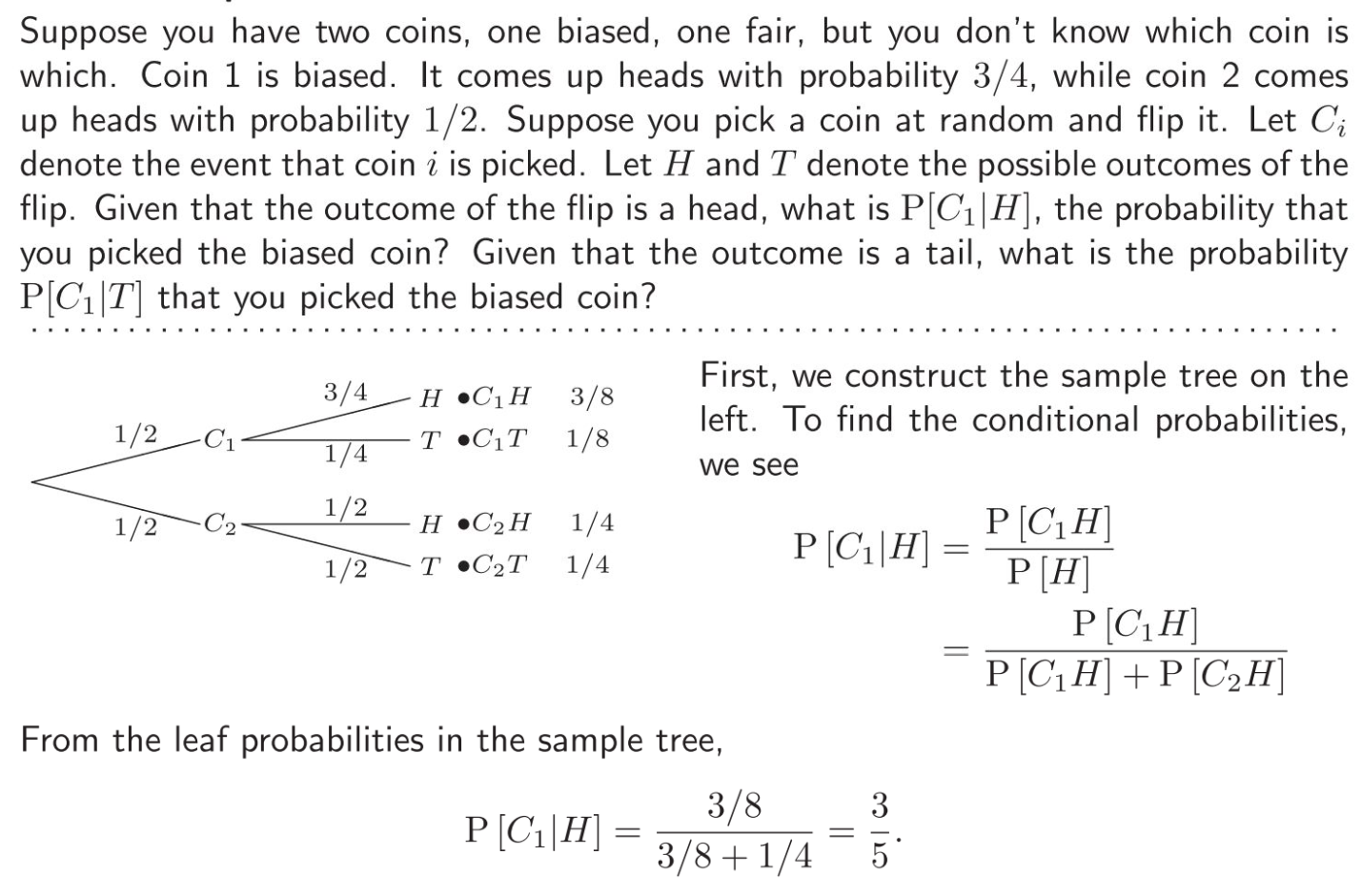
From this we can see that tree diagrams help us to calculate probabilities of sequential events.
Tree diagrams display the outcomes of the subexperiments in a sequential experiment. The labels of the branches are probabilities and conditional probabilities. The probability of an outcome of the entire experiment is the product of the probabilities of branches from the root of the tree to a leaf.
Many experiments will consist of what we call subexperiments. The procedure followed for each subexperiment may depend on the results of the previous subexperiments.
In doing this we will assemble outcomes into different partitions, starting at the root of the tree. From there we branch (and label according probabilities) based on the probabilities of each outcome.
Section 2.2 - Counting Methods
In all application of probability theory, it should be important to understand the sample space of an experiment.
The methods in this section will help determine the number of outcomes in the sample space of an experiment.
Theorem 2.1
An experiment consists of two subexperiments. If one subexperiment has \(k\) outcomes and the other subexperiment has \(n\) outcomes, then the experiment has a total of \(nk\) outcomes.
Theorem 2.2
The number of \(k\)-permutations of \(n\) distinguishable objects is:
\[(n)_k = n(n-1)(n-2)(n-3)\dots(n-k+1)=\frac{n!}{(n-k)!}\]
Something that might help to remember permutations is that a permutation depends on the order in which the elements are in whereas a combination does not depend on the order.
For example, think if we had 100 students. Imagine that we want to put any 50 of those students into a line. This means that the number of different permutations (arrangements) of that line is equal to \(\frac{100!}{(100-50)!}=\frac{100!}{50!}\)
Theorem 2.3
The number of ways to choose k objects out of n distinguishable objects is:
\[\begin{pmatrix} n\\k \end{pmatrix} = \frac{(n)_k}{k!} = \frac{n!}{k!(n-k)!}\]
Sometimes this is called a combination where the order in which items are picked does not matter, as opposed to the permutation.
Definition 2.1: \(n\) choose \(k\)
For any integer \(n \geq 0\), we define
\[\begin{pmatrix} n \\ k \end{pmatrix} = \begin{cases} \frac{n!}{k!(n-k)!} & k = 0, 1, \dots, n, \\ 0 & \text{otherwise}. \end{cases}\]
Theorem 2.4
Given \(m\) distinguishable object, there are \(m^n\) ways to choose with replacement an ordered sample of \(n\) objects.
Theorem 2.5
for \(n\) repetitions of a subexperiment with sample space \(S_{sub} = \lbrace s_0, \dots, s_{m-1} \rbrace\), the sample space \(S\) of the sequential experiment has \(m^n\) outcomes
Theorem 2.6
The number of observation frequencies for n subexperiments with sample space \(S = \lbrace 0, 1 \rbrace\) with 0 appearing \(n_)\) times and 1 appearing \(n_1=n-n_0\) times is \(\begin{pmatrix} n \\ n_1 \end{pmatrix}\)
Theorem 2.7
For \(n\) repetitions of a subexperiment with sample space \(S = \{s_0,\dots,s_{m-1}\}\) the number of length \(n = n_0 + \dots + n_{m-1}\) observation sequences with \(s_i\) appearing \(n_i\) times is
\[\begin{pmatrix} n \\ n_0,\dots,n_{m-1} \end{pmatrix} = \frac{n!}{n_0!n_1!\dots n_{m-1}!}\]
Independent Trials
Theorem 2.8
The probability of \(n_0\) failures and \(n_1\) successes in \(n=n_0+n_1\) independent trials is:
\[P[E_{n_0}, n_1] = \begin{pmatrix} n \\ n_1 \end{pmatrix} = (1-p)^{n-n_1}p^{n_1} = \begin{pmatrix} n \\ n_0 \end{pmatrix} (1-p)^{n_0}p^{n-n_0}\]
Chapter 3 - Discrete Random Variables
Definition - Discrete Variables - A random variable assigns numbers to outcomes in the sample space of an experiment.
A probability model always begins with an experiments. And each of the random variables is directly related to the experiment.
There are 3 types of relationships
- The random variable is the observation
- The random variable is a function of the observation
- The random variable is a function of another random variable.
Throughout most of the book probability is examined in models that assign numbers to the outcomes of the sample space.
When we observe the observation we call it a random variable. Typically in our notation the name of our random variable is a capital letter. e.g. \(X\).
The set of possible values for \(X\) is the range of \(X\)
Since we often consider multiple variables at a time, we denote the range of a random variable by the letter \(S\) with a subscript that is the name of the random variable.
Thus, \(S_X\) is the range of the random variable \(X\), \(S_Y\) is the range of the random variable \(Y\) and so on…
Definition 3.1
Random Variable consists of an experiment with a probability measure \(P[.]\) defined on a sample space \(S\) and a function that assigns a real number to each outcome in the sample space of the experiment.
A note on notation:
-
On occasion should we need to identify the random variable \(X\) with respect to a sample outcome, then we define this as \(X(s)\). (In other words we define a function which relates the value of X to the outcomes - X is a function of \(s\), the outcome)
-
Sometimes we will write \(\{ X = x\}\)to emphasize that there is a set of sample points \(s \in S\) for which \(X(s) = x\).
We can then adopt the following shorthand notation:
\[\{X = x\} = \{s\in S \ \vert\ X(s) = x\}\]
Definition 3.2
\(X\) is a discrete random variable if the range of \(X\) is a countable set
\[S_X = \{x_1,x_2,\dots\}\]Definition 3.3
Probability Mass Function (PMF) - The probability mass function of the discrete random variable X is
\[P_X(x) = P[X=x]\]
A way of putting this is that for a certain discrete random variable which is described by \(P_X\), then saying \(P_X(x)\) is the probability of the event in which that \(x\) occurs, or in other words it is \(P[X=x]\), where the big \(X\) is the random variable and \(P\) simply denotes that it is the PMF function.
Theorem 3.1
For a discrete random variable \(X\) with a PMF of \(P_X(x)\) and range \(S_X\)
- \[\text{For any } x, P_X(x) \geq 0\]
- \[\sum\limits_{x\in S_X} P_X(x) = 1\]
- For any event \(B\subset S_X\), the probability that \(X\) is in the set \(B\) is
- \[P[B] = \sum\limits_{x\in B} P_X(x)\]
To put this into words we can say that to calculate the probability of an event, \(B\), then it is the sum total probability of all outcomes for \(P_X\) which are contained within \(B\)
Families of Random Variables
- In practical applications, certain types of random variables appear over and over across many experiments.
- In each of these families (types) the PMF of all the random variables will have the same mathematical form
- Differ only in values of one or two parameters
- Depending on family, each PMF will contain only 1-2 parameters
- If we assign numbers to the parameters we can obtain a specific variable.
- Typical nomenclature for a family consists of the family name followed by one or two parameters in parentheses.
Example: binomial(n, p) refers in general to the family of binomial random variables
Binomial(7, 0.1) refers to the binomial random variable with parameters \(n=7\) and \(p = 0.1\)
Definition 3.4
X is a Bernoulli (p) random variable if the PMF of X has the form
\[P_X(x) = \begin{cases} 1-p , & x = 0 \\ p , & x = 1 \\ 0, & \text{otherwise} \end{cases}\]
- \(X =\) The number of successes in a single trial.
Definition 3.5 Geometric (p) Random Variable
X is a geometric (p) random variable if the PMF of X has the form
\[P_X(x) = \begin{cases} p(1-p)^{x-1}, & x = 0 \\0, & \text{otherwise} \end{cases}\]
- \(X =\) Number of trials until (up to and including) the first success
Definition 3.6 Binomial (n, p) Random Variable
X is a binomial (n, p) random variable if the PMF of X has the form
\[P_X(x) = \begin{pmatrix} n \\ x \end{pmatrix} p^x(1-p)^{n-x}\]
Where \(0 < p < 1\) and \(n\) is an integer such that \(n \geq 1\)
- \(X =\) the number of successes in n trials
Definition 3.7 Pascal (k, p) Random Variable
X is a pascal (k, p) random variable if the PMF of X has the form:
\[P_X(x) = \begin{pmatrix} x-1 \\ k-1 \end{pmatrix} p^k(1-p)^{x-k}\]
Where \(0 < p < 1\) and k is an integer such that \(k \geq 1\)
- \(X =\) the number of trials until the \(k^{th}\) success
If \(k = 1\) then x is geometric.
- Bernoulli (p) = number successes in 1 trial
- Geometric (p) = number of trials until 1st success
- Binomial (n, p) = number of successes in n trials
- Pascal (k, p) = number of trials until k successes
| Name of Random Variable | Description of variable | PMF Function |
|---|---|---|
| Bernoulli | number successes in 1 trial | \(P_X(x) = \begin{cases} 1-p , & x = 0 \\ p , & x = 1 \\ 0, & \text{otherwise} \end{cases}\) |
| Geometric | number of trials until 1st success | \(P_X(x) = \begin{cases} p(1-p)^{x-1}, & x = 0 \\0, & \text{otherwise} \end{cases}\) |
| Binomial | number of successes in n trials | \(P_X(x) = \begin{pmatrix} n \\ x \end{pmatrix} p^x(1-p)^{n-x}\) |
| Pascal | number of trials until k successes | \(P_X(x) = \begin{pmatrix} x-1 \\ k-1 \end{pmatrix} p^k(1-p)^{x-k}\) |
Definition 3.8 Discrete Uniform \((k, l)\) Random Variable
X is a discrete uniform \((k, l)\) random variable if the PMF of X has the form:
\[P_X(x) = \begin{cases} \frac{1}{l - k + 1},\ x=k, k+1, k+2\dots \\ 0, & \text{otherwise} \end{cases}\]
- X is uniformly distributed between \(k\) and \(l\).
Definition 3.9 Poisson (\(\alpha\)) Random Variable
X is a poisson (\(\alpha\)) random variable if the PMF of X has the form
\[P_X(x) = \begin{cases} \frac{\alpha^xe^{-\alpha}}{x!}, x=0,1,2\cdots \\0, & \text{otherwise} \end{cases}\]
- Call the phenomena of interest an arrival.
- Poisson model specifies an average rate.
- \(\lambda\) arrivals per second, over a time interval of \(T\) seconds.
- The number of arrivals \(X\) has a Poisson PMF with \(\alpha = \lambda T\)
Section 3.4 - Cumulative Distribution Function (CDF)
Like the PMF, the CDF of a random variable X expresses the probability model of an experiment as a mathematical function. The function is the probability \(P[X \leq x]\) for every number \(x\).
The cumulative distribution function (CDF) of a random variable, X, is
\[F_X(x) = P[X \leq x]\]Theorem 3.2
- \(F_X(\infty) = P[X \leq \infty] = 1\) - The probability which X is less than infinity.
- \(F_X(-\infty) = P[X \leq -\infty] = 0\) - The probability which X is less than infinity.
- For all \(x' \geq x, F_X(x') \geq F_X(x)\)
- For \(x_i \in S_X\) and \(\epsilon\), and arbitrarily small positive number
- \[F_X(x_i) - F_X(x_i - \epsilon) = P_X(x_i)\]
- \(F_X(x) = F_X(x_i)\) for all x such that \(x_i \leq x < x_{i+1}\)
Theorem 3.3
For all \(b \geq a\)
\[F_X(b) - F_X(a) = P[a < X \leq b]\]
In other words, to find the probability of an event between two values, you can simply subtract the values of the CDF at \(a\) and \(b\) because it is the sum total probability up to each of those points, subtracting them results in only the probability of values between \(a\) and \(b\).
Definition 3.13 Expected Value
The expected value of \(X\) is
\[E[X]=\mu_X = \sum\limits_{x\in S_X}^\ xP_X(x)\]This is sometimes referred to as the mean of a random variable or function
Theorem 3.4
The Bernoulli \(p\) random variable \(X\) has the expected value \(E[X]=p\)
Theorem 3.5
The geometric random variable \(X\) has the expected value \(E[X]=\frac{1}{p}\)
Theorem 3.6
The Poisson (\(\alpha\)) random variable in definition 3.9 has the expected value \(E[X]=\alpha\)
Theorem 3.7
1. For the binomial \((n, p)\) random variable \(X\) of definition 3.6
\[E[X] = np\]2. For the pascal \((k, p)\) random variable \(X\) of definition 3.7
\[E[X] = \frac{k}{p}\]3. For the discrete uniform \((k, l)\) random variable \(X\) of definition 3.7
\[E[X] = \frac{k+l}{2}\]Expected Value Table
| Function Type | Expected Value \(E[X]\) |
| Bernoulli | \(p\) |
| Geometric | \(\frac{1}{p}\) |
| Poisson | \(\alpha\) |
| Binomial | \(np\) |
| Pascal | \(\frac{k}{p}\) |
| Discrete Uniform | \(\frac{k + l}{2}\) |
Theorem 3.8
Perform \(n\) Bernoulli trials. In each trial let the probability of success be \(\frac{\alpha}{n}\) where \(\alpha > 0\) is a constant and \(n > \alpha\). Let the random variable \(K_n\) be the number of successes in \(n\) trials. As \(n\rightarrow \infty\) then \(P_{K_n}(k)\) converges to the PMF of a Poisson \((\alpha)\) random variable
Definition 3.11 Mode
A mode of random variable X is a number \(x_{mod}\) satisfying \(P_X(x_{mod}) \geq P_X(x)\) for all x
Definition 3.12 Median
A median \(x_{med}\) of random variable X is a number that satisfies these properties
- \[P[X \leq x_{med}]\geq \frac{1}{2}\]
- \[P[X\geq x_{med}] \geq \frac{1}{2}\]
Functions of a Random Variable
Definition 3.14
Each sample value y of a derived random variable Y is a mathematical function \(g(x)\) of a sample value x of another random variable X. We adopt the notation \(Y = g(X)\) to describe the relationship of the two random variables.
Definition 3.9
For a discrete random variable X, the PMF of \(Y=g(X)\) is
\[P_Y(y)=\sum\limits_{X:g(x)=y}^\ P_X(x)\]
Expected Value of a Derived Random Variable
Theorem 3.10
Given a random variable X with the PMF \(P_X(x)\) and derived random variable \(Y=g(X)\), the expected value of \(Y\) is
\[E[Y] = \mu_Y= \sum\limits_{x\in S_X}^\ g(x) P_X(x)\]
Theorem 3.11
For any random variable X,
\[E[X-\mu_X] = 0\]
Theorem 3.12
For any random variable X,
\[E[aX + b] = aE[X] + b\]
Variance and Standard Deviation
Definition 3.15 Variance
The variance of a random variable X is:
\[Var[X] = E[(X-\mu_X)^2]\]
You might have heard variance before as the square of standard deviation (\(\sigma\)). Thus follows the next definition.
Definition 3.16 Standard Deviation
The standard deviation of a random variable X is:
\[\sigma_X = \sqrt{Var[X]}\]
Theorem 3.13
In the absence of observations, the minimum mean square error estimate of random variable X is:
\[\hat{x} = E[X]\]
Theorem 3.14
\[Var[X] = E[X^2] - \mu_x^2 = E[X^2] - (E[X])^2\]
Theorem 3.17
For the Random variable, X
a. The nth moment is \(E[X^n]\) b. The nth central moment is \(E[(X-\mu_X)^n]\)
Theorem 3.15
\[Var[aX + b] = a^2 Var[X]\]
Theorem 3.16
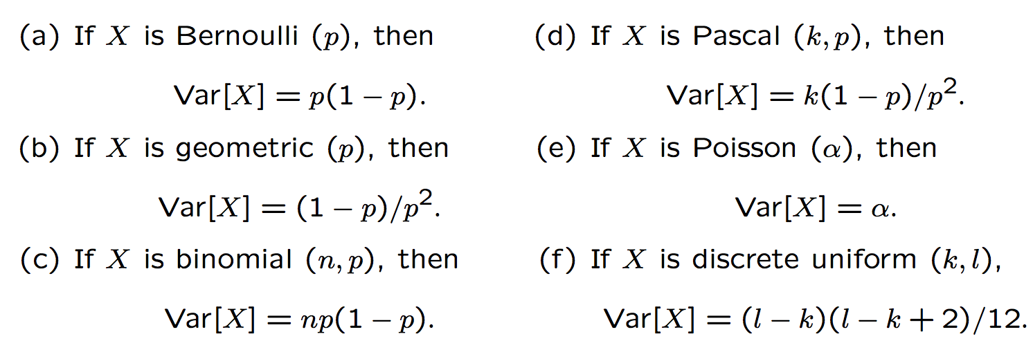
Variance Table
| Function Type | Variance \(Var[X]\) |
| Bernoulli | \(p(1-p)\) |
| Geometric | \(\frac{1-p}{p^2}\) |
| Poisson | \(\alpha\) |
| Binomial | \(np(1-p)\) |
| Pascal | \(\frac{k(1-p)}{p^2}\) |
| Discrete Uniform | \(\frac{(l-k)(l-k+2)}{12}\) |
Full Table of Discrete Random Variables
| Name of Random Variable | Description of variable | PMF Function | Expected Value- \(E[X]\) | Variance - \(Var[X]\) |
|---|---|---|---|---|
| Bernoulli | number successes in 1 trial | \(P_X(x) = \begin{cases} 1-p , & x = 0 \\ p , & x = 1 \\ 0, & \text{otherwise} \end{cases}\) | \(p\) | \(p(1-p)\) |
| Geometric | number of trials until 1st success | \(P_X(x) = \begin{cases} p(1-p)^{x-1}, & x = 0 \\0, & \text{otherwise} \end{cases}\) | \(\frac{1}{p}\) | \(\frac{1-p}{p^2}\) |
| Binomial | number of successes in n trials | \(P_X(x) = \begin{pmatrix} n \\ x \end{pmatrix} p^x(1-p)^{n-x}\) | \(np\) | \(np(1-p)\) |
| Pascal | number of trials until k successes | \(P_X(x) = \begin{pmatrix} x-1 \\ k-1 \end{pmatrix} p^k(1-p)^{x-k}\) | \(\frac{k}{p}\) | \(\frac{k(1-p)}{p^2}\) |
| Poisson | Probability of x arrivals in T seconds | \(P_X(x) = \begin{cases} \frac{\alpha^xe^{-\alpha}}{x!}, x = 0, 1, 2\dots \\ 0,\text{otherwise} \\ \end{cases}\) | \(\alpha\) | \(\alpha\) |
| Discrete Uniform | Probability of any value between k and l | \(P_X(x) = \begin{cases} \frac{1}{l - k + 1},\ x=k, k+1, k+2\dots \\ 0, \text{otherwise} \end{cases}\) | \(\frac{k + l}{2}\) | \(\frac{(l-k)(l-k+2)}{12}\) |
Chapter 4 - Continuous Random Variables
Example:
Imagine a circle with an infinite amount of points around the circle. If we were to pick any one point at random. What would the probability of picking that point be?
So what if we ask, what is the probability we choose the point of \(x = 0.25\), or \(P[X=0.25]\).
Well, it turns out, the answer, \(P[X=0.25] = 0\). This will lead us into the first section
Section 4.1 - Continuous Sample Space
In a continuous sample space, there are an infinite number of points you could choose. But the probability of picking a single point is zero.
Section 4.2 - The Cumulative Distribution Function
Definition 4.1 - Cumulative Distribution Function (CDF)
\[F_X(x) = P [ X \leq x]\]
Recall this from previous sections. It applies to continuous random variables as the probability of any single event is 0, but for all values up to and including a single value is how we calculate the probability of a continuous function.
Theorem 4.1
For any random variable X
- \(F_X(-\infty) = 0\) – \(P[X \leq -\infty] = 0\)
- \(F_X(\infty) = 1\) – \(P[X \leq \infty] = 0\)
- \[P[x_1 \leq X \leq x_2] = F_X(x_2) - F_X(x_1)\]
Definition 4.2 - Continuous Random Variable
\(X\) is a continuous random variable if the CDF \(F_X(x)\) is a continuous function
Section 4.3 - The Probability Density Function
The probability density function (PDF) of a continuous random variable X is:
\[f_X(x) = \frac{dF_X(x)}{dx}\]
This function is simply defined as the derivative of the CDF function for a continuous random variable.
Theorem 4.2
For a continuous random variable X with a PDF of \(f_X(x)\)
- \[f_X(x) \geq 0 \text{ for all } x\]
- \[F_X(x) = \int\limits_{-\infty}^x f_X(u)du\]
- \[\int\limits_{-\infty}^{\infty} f_X(x)dx = 1\]
Theorem 4.3
\[P[x_1 < X \leq x_2] = \int\limits_{x_1}^{x_2} f_X(x)dx\]
Section 4.4 - Expected Values
The expected value of a continuous random variable X is:
\[E[X] = \int\limits_{-\infty}^{\infty} xf_X(x)dx\]
Theorem 4.4
The expected value of a function \(g(X)\) of a random variable X is:
\[E[g(x)] = \int\limits_{-\infty}^{\infty} g(x)f_X(x)dx\]
Theorem 4.5
For any random variable \(X\)
- \[E[X-\mu_X] = 0\]
- \[E[aX + b] = aE[X] + b\]
- \[Var[X] = E[X^2] - \mu_X^2\]
- \[Var[aX + b] = a^2Var[X]\]
Section 4.5 - Families of Continuous Random Variables
Definition 4.5 Uniform Random Variable
X is a uniform (a, b) random variable if the PDF of X is
\[f_X(x) = \begin{cases} \frac{1}{b-a} & a \leq x < b, \\ 0 & \text{otherwise} \end{cases}\]
Where the condition is that the parameter \(b > a\)
Theorem 4.6
If X is a uniform (a, b) random variable
- The CDF of X is: \(F_X(x) = \begin{cases} 0 & x \leq a \\ \frac{x-a}{b-a} & a < x \leq b \\ 1 & x > b \end{cases}\)
- The expected value of X is \(E[X] = \frac{b + a}{2}\)
- The variance of X is \(Var[X] = \frac{(b-a)^2}{12}\)
Theorem 4.7
Let X be a uniform \((a, b)\) random variable, where a and b are both integers. Let \(K = \lceil X\rceil\). Then K is a discrete uniform \((a+1, b)\) random variable.
Note that \(\lceil X \rceil\) is the “ceiling” of the range of X, or the greatest value in the set
Definition 4.6 - Exponential Random Variable
X is an exponential (\(\lambda\)) random variable if the PDF of X is:
\[f_X(x) = \begin{cases} \lambda e^{-\lambda x} & x \geq 0 \\ 0 & \text{otherwise} \end{cases}\]
Theorem 4.8
If X is an exponential (\(\lambda\)) random variable
- The CDF of X is: \(F_X(x) = \begin{cases} 1-e^{-\lambda x} & x \geq 0 \\ 0 & \text{otherwise} \end{cases}\)
- The expected value of X is \(E[X] = \frac{1}{\lambda}\)
- The variance of X is \(Var[X] = \frac{1}{\lambda^2}\)
Theorem 4.9
If X is an exponential (\(\lambda\)) random variable, then \(K = \lceil X \rceil\) is a geometric (p) random variable with \(p = 1 - e^{-\lambda}\)
Definition 4.7 - Erlang Random Variable
X is an Erlang (\(n, \lambda\)) random variable if the PDF of X is:
\[f_X(x) = \begin{cases} \frac{\lambda^2 x^{n-1}e^{-\lambda x}}{(n-1)!} & x > 0 \\ 0 & \text{otherwise} \end{cases}\]
where the parameter of \(\lambda > 0\) and the parameter \(n \geq 1\) is an integer.
Theorem 4.10
If X is an Erlang (\(n, \lambda\)) random variable, then
- \[E[X] = \frac{n}{\lambda}\]
- \[Var[X] = \frac{n}{\lambda^2}\]
Theorem 4.11
Let \(K_{\alpha}\) denote a Poisson (\(\alpha\)) random variable. For any \(x > 0\), the CDF of an Erlang (\(n, \lambda\)) random variable X, satisfies
\[F_X(x) = 1 - F_{K_{\lambda x}}(n-1) = \begin{cases} 1 - \sum\limits_{k=0}^{n-1} \frac {(\lambda x)^k e^{-\lambda x}}{k!} & x \geq 0 \\ 0 & \text{otherwise} \end{cases}\]
Section 4.6 - Gaussian Random Variables
Definition 4.8 - Gaussian Random Variable
\(X\) is a Gaussian \((\mu, \sigma)\) random variable if the PDF of \(X\) is:
\[f_X(x) = \frac{1}{\sqrt{2\pi\sigma^2}}e^{-(x-\mu)^2/2\sigma^2}\]
The parameter \(\mu\) can be any real number and the parameter \(\sigma > 0\)
Theorem 4.12
If X is a Gaussian \((\mu, \sigma)\) random variable:
\(E[X] = \mu\) and \(Var[X] = \sigma^2\)
Theorem 4.13
If X is a Gaussian \((\mu, \sigma)\) random variable, \(Y=aX + b\) is Gaussian \((a\mu + b, a\sigma)\)
Definition 4.9 - Standard Normal Random Variable
The standard normal random variable \(Z\) is the Gaussian (0, 1) random variable
Definition 4.10 - Standard Normal CDF
The CDF of the standard normal random variable Z is:
\[\Phi (z) = \frac{1}{\sqrt{2\pi}} \int\limits_{-\infty}^z e^{-u^2/2}du\]
Theorem 4.14 - If X is a Gaussian \((\mu, \sigma)\) random variable, then the CDF of X is:
\[F_X(x) = \Phi (\frac{x-\mu}{\sigma})\]
And the probability that X is in the interval of (a, b] (includes b, excludes a):
\[P[a < X \leq b] = \Phi (\frac{b-\mu}{\sigma}) - \Phi (\frac{a - \mu}{\sigma})\]
Theorem 4.15
\[\Phi(-z) = 1 - \Phi(z)\]
Definition 4.11 - Standard Normal Complementary CDF
The standard normal complementary CDF is:
\[Q(z) = P[Z > z] = \frac{1}{\sqrt{2\pi}} \int\limits_z^\infty e^{-e^2/2}du = 1 - \Phi (z)\]
Another way of looking at is is that \(Q(z) = \Phi (-z) = 1-\Phi (z)\)
Section 4.7 - Delta Functions, Mixed Random Variables
Definition 4.12 - Unit Step Function
The unit step function is:
\[u(x) = \begin{cases} 0, x < 0 \\ 1, x \geq 0 \end{cases}\]
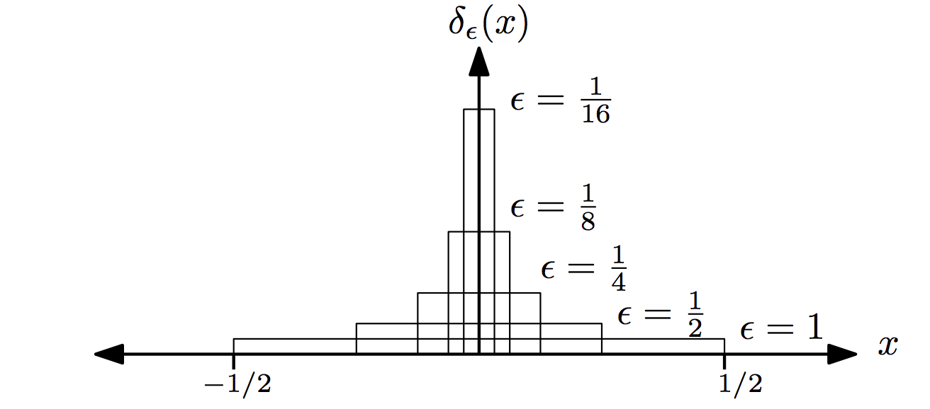
Definition 4.12 - Unit Impulse (Delta) Function
Let
\[d_\epsilon (x) = \begin{cases} 1/\epsilon, & -\epsilon/2 \leq x \leq \epsilon/2 \\ 0 , & \text{otherwise} \end{cases}\]
Then the unit impulse function is
\[\delta (x) = \lim\limits_{\epsilon\rightarrow 0} d_\epsilon(x)\]
Now as \(\epsilon\) approaches the delta function \(\delta (x)\) for each \(\epsilon\) the area under the curve of the \(d_{\epsilon} (x)\) equals 1
Theorem 4.16
For any continuous function g(x)
\[\int\limits_{-\infty}^{\infty} g(x)\delta (x-x_0)dc = g(x_0)\]
Theorem 4.17
\[\int\limits_{-\infty}^{x} \delta(v) dv = u(x)\]
Chapter 5 - Multiviews and Pairs of Random Variables
Pairs of Random Variables
We should consider experiments that produce a collection of random variables \(X_1, X_2, \dots, X_n\).
A pair of random variables \(X\) and \(Y\) is the same as the two dimensional vector, \(\pmb{X} = [X, Y]'\) this way. Since the components of this vector are both random variables we call \(\pmb{X}\) a random vector.
Definition 5.1 - Joint Cumulative Distribution Function (CDF)
The joint cumulative distribution function of random variables \(X\) and \(Y\) is
\[F_{X,Y}(x, y) = P[X \leq x, Y \leq y]\]
So if you can imagine a two dimensional graph that the CDF represents the probability of being within a rectangular region which the point that is picked is \(\leq\) x and y
Theorem 5.1
For any pair of random variables \(X, Y\)
- \[0 \leq F_{X,Y} \leq 1\]
- \[F_{X,Y}(\infty, \infty) = 1\]
- \[F_{X}(x) = F_{X,Y}(x, \infty)\]
- \[F_{Y}(y) = F_{X,Y}(\infty, y)\]
- \[F_{X,Y}(x, -\infty) = 0\]
- \[F_{X,Y}(-\infty, y) = 0\]
- If \(x \leq x_1 \text{ and } y \leq y_1\) then
- \[F_{X,Y}(x, y) \leq F_{X,Y}(x_1, y_1)\]
Theorem 5.2
\[P[x_1 \leq X \leq x_2, y_1 \leq Y \leq y_2] = F_{X,Y}(x_2, y_2) - F_{X,Y}(x_2, y_1) - F_{X,Y}(x_1, y_2) + F_{X,Y}(x_1, y_1)\]
Section 5.2 - Joint Probability Mass Function (PMF)
Definition 5.2 - Joint PMF
The joint PMF of discrete random variables \(X\) and \(Y\) is
\[P_{X,Y}(x, y) = P[X=x, Y = y]\]
Theorem 5.3 For discrete random variables \(X\) and \(Y\) and any set \(B\) in the \(X, Y\) plane, the probability of the event \(\{(X, Y) \in B\}\) is
\[P[B] = \sum\limits_{(x, y) \in B} P_{X, Y}(x, y)\]
Section 5.3 - Marginal PMF
Theorem 5.4
For Discrete random variables X and Y with joint PMF \(P_{X, Y}(x, y)\)
- \[P_X(x) = \sum\limits_{y\in S_Y} P_{X, Y}(x, y)\]
- \[P_Y(y) = \sum\limits_{x\in S_x} P_{X, Y}(x, y)\]
Section 5.4 Joint Probability Density Function
Definition 5.3 - Joint PDF
The joint PDF of the continuous random variables \(X\) and \(Y\) is a function \(f_{X, Y}(x, y)\) with the property
\[F_{X, Y}(x, y) = \int\limits_{-\infty}^x\int\limits_{-\infty}^y f_{X, Y}(u, v)du\cdot dv\]
Theorem 5.5
\[f_{X, Y}(x, y) = \frac{\partial^2F_{X, Y}(x, y)}{\partial x \partial y}\]
Theorem 5.6
A joint PDF \(f_{X, Y}(x, y)\) has the following properties corresponding to the first and second axioms of probability
- \[f_{X, Y}(x, y) \geq 0 \text{ for all } (x, y)\]
- \[\int\limits_{-\infty}^\infty\int\limits_{-\infty}^\infty f_{X, Y}(x, y) dx\cdot dy = 1\]
Theorem 5.7
The probability of the continuous random variables (X, Y) are in A is:
\[P[A] = \iint_A f_{X, Y}(x, y)dx\cdot dy\]
Section 5.5 - Marginal PDF
Theorem 5.8
If \(X\) and \(Y\) are random variables with joint PDF \(f_{X,Y}(x, y)\)
- \[f_X(x) = \int\limits_{-\infty}^\infty f_{X,Y}(x, y)dy\]
- \[f_Y(y) = \int\limits_{-\infty}^\infty f_{X,Y}(x, y)dx\]
Section 5.6 - Independent Random Variables
Definition 5.4 - Independent Random Variables
Random variable \(X\) and \(Y\) are independent if and only if the following are true:
For discrete random variables:
\[P_{X,Y}(x, y) = P_X(x)P_Y(y)\]
For continuous random variables:
\[f_{X,Y}(x, y) = f_X(x)f_Y(y)\]
Section 5.7 - Expected Value of a Function of Two Random Variables
Theorem 5.9
For random variables \(X\) and \(Y\) the expected value of \(W = g(X, Y)\) is:
For discrete random variables:
\[E[W] = \sum\limits_{x\in S_X} \sum\limits_{y\in S_Y} g(x, y)P_{X, Y}(x, y)\]
For continuous random variables:
\[E[W] = \int\limits_{-\infty}^\infty \int\limits_{-\infty}^\infty g(x, y) f_{X, Y}(x, y)dx\cdot dy\]
Theorem 5.10
\[E[a_1g_1(X, Y) + \dots + a_ng_n(X, Y)] = a_1E[g_1(X, Y)] + \dots + a_nE[g_n(X, Y)]\]
Theorem 5.11
For any two random variables X and Y
\[E[X + Y] = E[X] + E[Y]\]
Theorem 5.12
The variance of the sum of two random variables is:
\[Var[X + Y] = Var[X] + Var[Y] + 2E[(X-\mu_X)(Y-\mu_Y)]\]
Definition 5.5 - Covariance
The covariance of two random variables \(X\) and \(Y\) is:
\[Cov[X, Y] = E[(X-\mu_X)(Y-\mu_Y)]\]
Definition 5.6 - Correlation Coefficient
The correlation coefficient of two random variables X and Y is:
\[\rho_{X, Y} = \frac{Cov[X, Y]}{\sqrt{Var[X]Var[Y]}} = \frac{Cov[X,Y]}{\sigma_x\sigma_y}\]
Theorem 5.13
If \(\hat{X} = aX + b\) and \(\hat{Y} = cY + d\), then
- \[\rho_{\hat{X}, \hat{Y}} = \rho_{X, Y}\]
- \[Cov[\hat{X}, \hat{Y}] = ac\cdot Cov[X, Y]\]
Theorem 5.14
\[-1 < \rho_{X, Y} \leq 1\]
Theorem 5.15
If X and Y are random variables such that \(Y=aX + b\) then:
\[\rho_{X, Y} = \begin{cases} -1, & a < 0 \\ 0, & a = 0 \\ 1, & a > 0 \\ \end{cases}\]
Definition 5.7 - Correlation
The correlation of two variables \(X\) and \(Y\) is
\[r_{X, Y} = E[XY]\]
Theorem 5.16
-
\(Cov[X, Y] = r_{X, Y} - \mu_X\mu_Y\).
-
\(Var[X + Y] = Var[X] + Var[Y] + 2Cov[X, Y]\).
-
If \(X = Y\), \(Cov[X, Y] = Var[X] = Var[Y]\) and \(r_{X, Y} = E[X^2] = E[Y^2]\)
Definition 5.8 - Orthogonal Random Variables
Random variables X and Y are orthogonal if \(r_{X, Y} = 0\)
Definition 5.9 - Uncorrelated Random Variables
Random variables \(X\) and \(Y\) are uncorrelated if \(Cov[X, Y] = 0\)
Theorem 5.17
For independent random variables X and Y
- \[E[g(X)h(Y)] = E[g(X)]E[h(Y)]\]
- \[r_{X, Y} = E[XY] = E[X]E[Y]\]
- \[Cov[X, Y] = \rho_{X, Y} = 0\]
- \[Var[X + Y] = Var[X] + Var[Y]\]
Section 5.9 - Bivariate Gaussian Random Variables
Definition 5.10 - Bivariate Gaussian Random Variables
Random variables \(X\) and \(Y\) have bivariate Gaussian PDF with the parameters \(\mu_X\), \(\mu_Y\), \(\sigma_X > 0\), \(\sigma_Y > 0\), and that \(\rho_{X, Y}\) satisfying \(-1 < \rho_{X, Y} < 1\) if
\[f_{X, Y}(x, y) = \frac{ exp[ - \frac{ (\frac{x - \mu_X}{\sigma_X})^2 - \frac{2\rho_{X, Y}(x-\mu_X)(y-\mu_Y)}{\sigma_X\sigma_Y} + (\frac{y-\mu_Y}{\sigma_Y})^2 }{ 2(1-\rho_{X, Y}^2 ) } ] }{ 2\pi\sigma_X\sigma_Y\sqrt{1-\rho_{X, Y}^2} }\]
Theorem 5.18
If X and Y are bivariate Gaussian random variables in Definition 5.10, X is the Gaussian \((\mu_X, \sigma_X)\) and the random variable Y is the Gaussian \((\mu_Y, \sigma_Y)\) random variable:
- \[f_X(x) = \frac{1}{\sigma_X\sqrt{2\pi}}e^{-(x-\mu_X)^2/2\sigma_X^2}\]
- \[f_Y(y) = \frac{1}{\sigma_Y\sqrt{2\pi}}e^{-(y-\mu_Y)^2/2\sigma_Y^2}\]
Theorem 5.19
Bivariate Gaussian random variables X and Y in Definition 5.10 have the correlational coefficient \(\rho_{X, Y}\)
Theorem 5.20
Bivariate Gaussian random variables X and Y are uncorrelated if and only if they are independent
Theorem 5.21
If X and Y are bivariate Gaussian random variables with PDF given by definition 5.10 and \(W_1\) and \(W_2\) are given by the linearly independent equations
- \[W_1 = a_1X + b_1Y\]
- \[W_2 = a_2X + b_2Y\]
Then, \(W_1\) and \(W_2\) are bivariate Gaussian random variables such that
- \(E[W_i] = a_i\mu_X + b_i\mu_Y\) where \(i=1, 2\)
- \(Var[W_i] = a_i^2\sigma_X^2 + b_i\sigma_Y^2 + 2a_ib_i\rho_{X, Y}\sigma_X\sigma_Y\) where \(i=1, 2\)
- \[Cov[W_1, W_2] = a_1a_2\sigma_X^2 + b_1b_2\sigma_Y^2 + (a_1b_2 + a_2b_1)\rho_{X, Y}\sigma_X\sigma_Y\]
Section 5.10 - Multivariate Probability Models
Definition 5.11 - Multivariate Joint CDF
The joint CDF of \(X_1, \dots ,X_n\) is:
\[F_{X_1, \dots , X_n}(x_1, \dots , x_n) = P[X_1 \leq x_1, \dots ,X_n \leq x_n]\]
Definition 5.12 - Multivariate Joint PMF
The joint PMF of the discrete random variables \(X_1, \dots ,X_n\) is:
\[P_{X_1, \dots , X_n}(x_1, \dots , x_n) = P[X_1 = x_1, \dots ,X_n = x_n]\]
Definition 5.13 - Multivariate Joint PDF
The joint PDF of the continuous random variables of \(X_1, \dots, X_n\) is:
\[f_{X_1, \dots , X_n}(x_1, \dots , x_n) = \frac{\partial^nF_{X_1, \dots ,X_n}(x_1, \dots ,x_n)}{\partial x_1\dots \partial x_n}\]
Theorem 5.22
if \(X_1,\dots ,X_n\) are discrete random variables that have a joint PMF \(P_{X_1, \dots , X_n}(x_1, \dots , x_n)\)
- \[P_{X_1, \dots , X_n}(x_1, \dots , x_n) \geq 0\]
- \[\sum\limits_{x_1\in S_{X_1}} \dots \sum\limits_{x_n\in S_{X_n}} P_{X_1, \dots , X_n}(x_1, \dots , x_n) = 1\]
Theorem 5.23
if \(X_1,\dots ,X_n\) are continuous random variables that have a joint PDF \(f_{X_1, \dots , X_n}(x_1, \dots , x_n)\)
- \[f_{X_1, \dots , X_n}(x_1, \dots , x_n) \geq 0\]
- \[F_{X_1, \dots , X_n}(x_1, \dots , x_n) = \int\limits_{-\infty}^{x_1} \dots \int\limits_{-\infty}^{x_n} f_{X_1, \dots , X_n}(u_1, \dots , u_n)du_1\dots du_n\]
- \[\int\limits_{-\infty}^{\infty} \dots \int\limits_{-\infty}^{\infty} f_{X_1, \dots , X_n}(x_1, \dots , x_n)dx_1\dots dx_n = 1\]
Theorem 5.24
The probability of an event A expressed in terms of the random variables \(X_1, \dots , X_n\) is:
Discrete:
\[P[A] = \sum\limits_{(x_1\dots x_n)\in A} P_{X_1,\dots ,X_n}(x_1,\dots ,x_n)\]
Continuous:
\[P[A] = \int\dots\int_A f_{X_1, \dots , X_n}(x_1, \dots , x_n)dx_1\dots dx_n\]
Theorem 5.25
For a joint PMF \(P_{X, Y, Z}(x, y, z)\) of discrete random variables \(W, X, Y, Z\) some marginal PMFs are:
- \[P_{X, Y, Z}(x, y, z) = \sum\limits_{w\in S_w} P_{W, X, Y, Z}(w, x, y, z)\]
- \[P_{W,Z}(w, z) = \sum\limits_{x\in S_x} \sum\limits_{y\in S_y} P_{W, X, Y, Z}(w, x, y, z)\]
Theorem 5.26
For a joint PDF \(f_{X, Y, Z}(x, y, z)\) of discrete random variables \(W, X, Y, Z\) some marginal PDFs are:
- \[f_{W, X, Y}(w, x, y) = \int\limits_{-\infty}^\infty f_{W, X, Y, Z}(w, x, y, z)dz\]
- \[f_X(x) = \int\limits_{-\infty}^\infty\int\limits_{-\infty}^\infty\int\limits_{-\infty}^\infty f_{W, X, Y, Z}(w, x, y, z)dw\cdot dy\cdot dz\]
Definition 5.14 - N Independent Random Variables
Random variables \(X_1,\dots , X_n\) are independent if for all \(x_1, \dots , x_n\)
Discrete:
\[P_{X_1,\dots ,X_n}(x_1,\dots ,x_n) = P_{X_1}(x_1)P_{X_2}(x_2)\dots P_{X_n}(x_n)\]
Continuous
\[f_{X_1,\dots ,X_n}(x_1,\dots ,x_n) = f_{X_1}(x_1)f_{X_2}(x_2)\dots f_{X_n}(x_n)\]
Definition 5.15 - Independent and Identically Distributed (iid)
\(X_1,\dots , X_n\) are independent and identically distributed if:
Discrete:
\[P_{X_1,\dots ,X_n}(x_1,\dots ,x_n) = P_{X}(x_1)P_{X}(x_2)\dots P_{X}(x_n)\]
Continuous
\[f_{X_1,\dots ,X_n}(x_1,\dots ,x_n) = f_{X}(x_1)f_{X}(x_2)\dots f_{X}(x_n)\]
Chapter 6 - Probability Models of Derived Random Variables
Section 6.1 - PMF of a Function of Two Discrete Random Variables
Theorem 6.1
For discrete random variables X and Y, the derived random variable \(W = g(X, Y)\) has the PMF
\[P_W(w) = \sum\limits_{(x, y):g(x, y) = w} P_{X, Y}(x, y)\]
Section 6.2 - Functions Yielding Continuous Random Variables
Theorem 6.2
If \(W = aX\) where \(a > 0\) then \(W\) has a CDF and PDF of:
| CDF | |
| \(F_W(w) = F_X(w/a)\) | \(f_W(w)=\frac{1}{a}f_X(w/a)\) |
Theorem 6.3
Given that \(W = aX\) where \(a > 0\)
- If \(X\) is uniform \((b, c)\) then \(W\) is uniform \((ab, ac)\)
- If \(X\) is exponential \((\lambda)\) then \(W\) is exponential \((\lambda /a)\)
- If \(X\) is Erlang \((n, \lambda)\) then \(W\) is Erlang \((n, \lambda /a)\)
- If \(X\) is Gaussian \((\mu, \sigma)\) then \(W\) is Gaussian \((a\mu, a\sigma)\)
Theorem 6.4
Given that \(W = X + b\)
| CDF | |
| \(F_W(w) = F_X(w-b)\) | \(f_W(w) = f_X(w-b)\) |
Theorem 6.5
Let \(U\) be a uniform \((0, 1)\) random variable and let \(F(x)\) denote a cumulative distribution function with an inverse \(F^{-1}(u)\) defined for \(0 < u < 1\) the random variable \(X = F^{-1}(U)\) has CDF \(F_X(x) = F(x)\)
Section 6.4 - Continuous Function of Two Continuous Random Variables
Theorem 6.6
For continuous random variables \(X\) and \(Y\), the CDF of \(W = g(X, Y)\) is
\[F_W(w) = P[W \leq w] = \iint_{g(x, y) \leq w} f_{X, Y}(x, y) dxdy\]
Theorem 6.7
For continuous random variables \(X\) and \(Y\), the CDF of \(W = max(X, Y)\) is:
\[F_W(w) = F_{X, Y}(w, w, ) = \int\limits_{-\infty}^w \int\limits_{-\infty}^w f_{X, Y}(x, y) dx dy\]
Chapter 7 - Conditional Probability Models
Section 7.1 - Conditioning a Random Variable by an Event
Definition 7.1 - Conditional CDF
Given the event \(B\) with \(P[B] > 0\) the conditional cumulative distribution function of X is
\[F_{X|B}(x) = P[X \leq x | B]\]
Definition 7.2 - Conditional PMF Given an Event
Given the event B with \(P[B] > 0\), the conditional probability mass function of X is:
\[F_{X|B}(x) = P[X = x | B]\]
Definition 7.3 - Conditional PDF Given an Event
\[f_{X|B}(x) = \frac{dF_{X|B}(x)}{dx}\]
Theorem 7.1
For a random variable X and an event \(B \in S_X\) with \(P[B] > 0\), the conditional PDF of \(X\) given \(B\) is:
Discrete
\[P_{X|B}(x) = \begin{cases} \frac{P_X(x)}{P[B]} & x\in B \\ 0 & \text{otherwise} \\ \end{cases}\]
Continuous
\[f_{X|B}(x) = \begin{cases} \frac{f_X(x)}{P[B]} & x\in B \\ 0 & \text{otherwise} \\ \end{cases}\]
Theorem 7.2
For random variable \(X\) resulting from an experiment with partition
\[B_1,\dots,B_m\]Discrete: \(P_X(x) = \sum\limits_{i=1}^m P_{X\vert B_i}(x)P[B_i]\)
Continuous: \(f_X(x) = \sum\limits_{i=1}^m f_{X\vert B_i}(x)P[B_i]\)
Section 7.2 - Conditional Expected Value Given an Event
Theorem 7.3
| Discrete X | Continuous X |
| for any \(x\in B, P_{X\vert B}(x) \geq 0\) | for any \(x\in B, f_{X\vert B}(x) \geq 0\) |
| \(\sum\limits_{x\in B} P_{X\vert B}(x) = 1\) | \(\int_B f_{X\vert B}(x)dx=1\) |
| The conditional probability that X is in C: \(P[C\vert B] = \sum\limits_{x\in C} P_{X\vert B} (x)\) | The conditional probability that X is in the set C is: \(P[C\vert B] = \int_C f_{X\vert B} (x) dx\) |
Definition 7.4 - Conditional Expected Value
Discrete: \(E[X\vert B] = \sum\limits_{x\in B} x P_{X\vert B}(x)\)
Continuous: \(E[X\vert B] = \int\limits_{-\infty}^\infty x f_{X\vert B}(x)dx\)
Theorem 7.4
For a random variable \(X\) resulting from an experiment with partitions \(B_1,\dots,B_m\)
\[E[X] = \sum\limits_{i=1}^m E[X|B_i] \cdot P[B_i]\]
Theorem 7.5
The conditional expected value of \(Y=g(X)\) given the condition, \(B\) is:
Discrete: \(E[Y\vert B] = E[g(X)\vert B] = \sum\limits_{X\in B} g(x)P_{X\vert B} (x)\)
Continuous: \(E[Y\vert B] = E[g(X)\vert B] = \int\limits_{-\infty}^\infty g(x)f_{X\vert B} (x)\)
Section 7.3 - Condition Two Random Variables by an Event
Definition 7.6 - For discrete random variables \(X\) and \(Y\), and event, \(B\) with \(P[B] > 0\), the conditional joint PMF of \(X\) and \(Y\) given \(B\) is:
\[P_{X,Y\vert B}(x, y) = P[X=x, Y=y\vert B]\]
Theorem 7.6
For any event \(B\), a region of the \(X, Y\) plane with \(P[B] > 0\)
\[P_{X,Y \vert B} (x, y) = \begin{cases} \frac{P_{X, Y}(x, y)}{P[B]} & (x, y) \in B \\ 0 & \text{otherwise} \\ \end{cases}\]
Definition 7.7 - Conditional Joint PDF
Given an event \(B\) with \(P[B] > 0\), the conditional joint probability density function of \(X\) and \(Y\) is:
\[f_{X,Y\vert B}(x, y) = \begin{cases} \frac{f_{X, Y}(x, y)}{P[B]} & (x, y) \in B \\ 0 & \text{otherwise} \\ \end{cases}\]
Theorem 7.7 - Conditional Expected Value
For random variables \(X\) and \(Y\) and an event \(B\) of nonzero probability, the conditional expected value of \(W = g(X, Y)\) given \(B\) is:
Discrete: \(E[W\vert B] = \sum\limits_{x \in S_X} \sum\limits_{y \in S_Y} g(x, y) P_{X, Y \vert B} (x, y)\)
Continuous: \(E[W\vert B] = \int\limits_{-\infty}^\infty \int\limits_{-\infty}^\infty g(x, y) f_{X, Y \vert B} (x, y)\)
Section 7.4 - Condition by a Random Variable
Definition 7.8 - Conditional PMF
For any event \(Y = y\) such that \(P_{Y}(y) > 0\), the conditional PMF of \(X\) given \(Y=y\)
\[P_{X\vert Y}(x\vert y) = P[X=x \vert Y=y]\]
Theorem 7.8
For discrete random variables \(X\) and \(Y\) with joint PMF \(P_{X, Y}(x, y)\), and \(x\) and \(y\) such that \(P_{X}(x) > 0\) and \(P_Y(y) > 0\)
- \[P_{X\vert Y}(x\vert y) = \frac{P_{X, Y}(x, y)}{P_Y(y)}\]
- \[P_{Y\vert X}(y\vert x) = \frac{P_{X, Y}(x, y)}{P_X(x)}\]
Definition 7.9 - Conditional PDF
For y such that \(f_Y(y) > 0\), the conditional PDF of \(X\) given \({Y = y}\) is:
\[f_{X\vert Y}(x\vert y) = \frac{f_{X, Y}(x, y)}{f_Y(y)}\]
Theorem 7.9
For discrete random variables \(X\) and \(Y\) with joint PMF \(P_{X, Y}(x,y)\) and \(x\) and \(y\) such that \(P_X(x) > 0\) and \(P_Y(y) > 0\):
\[P_{X, Y}(x, y) = P_{Y\vert X}(y\vert x)P_X(x) = P_{X\vert Y}(x\vert y)P_Y(y)\]
Theorem 7.10
For continuous random variables \(X\) and \(Y\) with joint PDF \(f_{X, Y}(x,y)\) and \(x\) and \(y\) such that \(f_X(x) > 0\) and \(f_Y(y) > 0\):
\[f_{X, Y}(x, y) = f_{Y\vert X}(y\vert x)f_X(x) = f_{X\vert Y}(x\vert y)f_Y(y)\]
Theorem 7.11
If X and Y are independent:
Discrete: \(P_{X\vert Y}(x, y) = P_X(x)\), and \(P_{Y\vert X}(y\vert x) = P_Y(y)\)
Continuous: \(f_{X\vert Y}(x, y) = f_X(x)\), and \(f_{Y\vert X}(y\vert x) = f_Y(y)\)
Section 7.5 - Conditional Expected Value Given a Random Variable
Definition 7.10 - Conditional Expected Value of a Function
For any \(y \in S_Y\), the conditional expected value of \(g(X, Y)\) given \(Y = y\) is:
Discrete: \(E[g(X, Y)\vert Y = y] = \sum\limits_{x\in S_X} g(x, y) P_{X\vert Y}(x\vert y)\)
Continuous: \(E[g(X, Y)\vert Y = y] = \sum\limits_{-\infty}^\infty g(x, y) f_{X\vert Y}(x\vert y)\)
Theorem 7.12
For independent random variables \(X\) and \(Y\)
- \(E[X\vert Y=y] = E[X]\) for all \(y\in S_Y\)
- \(E[Y\vert X = x] = E[Y]\) for all \(x\in S_X\)
Definition 7.11 - Conditional Expected Value Function
The conditional expected value \(E[X\vert Y]\) is a function of random variable Y such that if \(Y = y\), then \(E[X\vert Y] = E[X\vert Y = y]\)
Theorem 7.13 - Iterated Expectation
\[E[E[X\vert Y]] = E[X]\]
Theorem 7.14
\[E[E[g(X)\vert Y]] = E[g(X)]\]
Theorem 7.15
If \(X\) and \(Y\) are the bivariate Gaussian random variables in Definition 5.10, the conditional PDF of \(Y\) given \(X\) is:
\[f_{Y\vert X} (y \vert x) = \frac{1}{\widetilde{\sigma_Y}\sqrt{2\pi}}e^{-(y-\widetilde{\mu}_Y(x))^2/2\widetilde{\sigma}_Y^2}\]
where, given \(X=x\), the conditional expected value and variance of \(Y\) are:
\[E[Y\vert X = x] = \widetilde{\mu}_Y(x) = \mu_Y + \rho_{X,Y}\frac{\sigma_Y}{\sigma_X}(x-\mu_X)\]
\[Var[Y\vert X = x] = \widetilde{\sigma}_Y^2 = \sigma_Y^2(1-\rho_{X, Y}^2)\]
Theorem 7.16
If \(X\) and \(Y\) are the bivariate Gaussian random variables in Definition 5.10, the conditional PDF of \(X\) given \(Y\) is:
\[f_{X\vert Y} (x\vert y) = \frac{1}{\widetilde{\sigma_X}\sqrt{2\pi}}e^{-(x-\widetilde{\mu}_x(y))^2/2\widetilde{\sigma}_X^2}\]
where, given \(Y=y\), the conditional expected value and variance of \(Y\) are:
\[E[X\vert Y = y] = \widetilde{\mu}_X(y) = \mu_X + \rho_{X,Y}\frac{\sigma_X}{\sigma_Y}(y-\mu_Y)\]
\[Var[X\vert Y = Y] = \widetilde{\sigma}_X^2 = \sigma_X^2(1-\rho_{X, Y}^2)\]
Chapter 9 - Sums of Random Variables
Section 9.1 - Expected Values of Sums
Theorem 9.1
For any set of random variables \(X_1, \dots, X_n\), the sum \(W_n = X_1 + \dots + X_n\) has the expected value:
\[E[W_n] = E[X_1] + E[X_2] + \dots + E[X_n]\]
Theorem 9.2
The variance of \(W_n = X_1 + \dots + X_n\) is:
\[Var[W_n] = \sum\limits_{i=1}^n Var[X_i] + 2\sum\limits_{i=1}^{n-1}\sum\limits_{j=i+1}^{n} Cov[X_i, X_j]\]
Theorem 9.3
When \(X_1 + \dots + X_n\) are uncorrelated:
\[Var[W_n] = Var[X_1] + \dots + Var[X_n]\]
Section 9.2 - Moment Generating Functions
Definition 9.1 - Moment Generating Function (MGF)
For a random variable \(X\), the moment generating function (MGF) of \(X\) is:
\[\phi_X(s) = E[e^{sX}]\]
Theorem 9.4
A random variable \(X\) with MGF \(\phi_X(s)\) has n-th moment:
\[E[X^n] = \frac{d^n\phi_X(s)}{ds^n} \text{at } s=0\]
Theorem 9.5
The MGF of \(Y = aX + b\) is \(\phi_Y(s) = e^{sb}\phi_X(as)\)
Section 9.3 - MGF of the Sum of Independent Random Variables
Theorem 9.6
For a set of independent random variables \(X_1, \dots, X_n\), the moment generating function of \(W = X_1 + \dots + X_n\) is:
\[\phi_W(s) = \phi_{X_1}(s)\phi_{X_2}(s) \dots \phi_{X_n}(s)\]
When \(X_1, \dots, X_n\) are iid, then each with MGF \(\phi_{X_i}(s) = \phi_X(s)\)
\[\phi_W(s) = [\phi_X(s)]^n\]
Theorem 9.7
If \(K_1, \dots, K_n\) are independent Poisson random variables, \(W = K_1,\dots, K_n\) is a Poisson random variable
Theorem 9.8
The sum of \(n\) independent Gaussian random variables \(W = X_1 + \dots + X_n\) is a Gaussian random variable
Theorem 9.9
If \(X_1, \dots, X_n\) are iid exponential (\(\lambda\)) random variables, then \(W = X_1 + \dots + X_n\) has the Erlang PDF:
\[f_W(w) = \begin{cases} \frac{\lambda^nw^{n-1}e^{-\lambda w}}{(n-1)!} & w \geq 0, \\ 0 & \text{otherwise} \\ \end{cases}\]
Theorem 9.12 - Central Limit Theorem
Given \(X_1, X_2, \dots,\) a sequence of iid random variables with expected value \(\mu_X\) and variance \(\sigma_X^2\), the CDF of \(Z_n = (\sum\limits_{i=1}^n X_i n\mu_X)/\sqrt{n\sigma_X^2}\)
\[\lim_{n\rightarrow\infty} F_{Z_n}(z) = \phi (z)\]
Definition 9.2 - Central Limit Theorem Approximation
Let \(W_n = X_1 + \dots + X_n\) be the sum of \(n\) iid random variables, each with \(E[X] = \mu_X\) and \(Var[X] = \sigma_X^2\). The central limit theorem approximation of the CDF of \(W_n\) is:
\[F_{W_n} (w) \approx \phi(\frac{w - n\mu_X}{\sqrt{n\sigma_X^2}})\]
Chapter 10 - The Sample Mean
Definition 10.1 - Sample Mean
For iid random variables \(X_1,\dots,X_n\) with PDF \(f_X(x)\), the sample mean of \(X\) is the random variable:
\[M_n(X) = \frac{X_1 + \dots + X_n}{n}\]
Theorem 10.1
The sample mean \(M_n(X)\) has the expected value and variance
Mean:
\[E[M_n(X)] = E[X]\]
Variance:
\[Var[M_n(X)] = \frac{Var[X]}{n}\]
A note on the sample variance: the the above theorem actually states that the sample mean \(M_n(X)\) converges to the expected value \(E[X]\) as the number of sample, \(n\) approaches \(\infty\)
Section 10.3 - The Laws of Large Numbers
Theorem 10.5 - Weak Law of Large Numbers (Finite Samples)
For any constant \(c > 0\)
\(P[\vert M_n(X) - \mu_X\vert \geq c] \leq \frac{Var[X]}{nc^2}\) \(P[\vert M_n(X) - \mu_X\vert < c] \geq 1- \frac{Var[X]}{nc^2}\)
Theorem 10.6 The Weak Law of Large Numbers (Infinite Samples)
If \(X\) has finite variance, then, for any constant \(c > 0\)
\(\lim\limits_{n\rightarrow\infty} P[\vert M_n(X) - \mu_X \vert \geq c] = 0\) \(\lim\limits_{n\rightarrow\infty} P[\vert M_n(X) - \mu_X \vert < c] = 1\)
Theorem 10.7
as \(n\rightarrow\infty\), the relative frequency \(\hat{P}_n(A)\) converges to \(P[A]\) for any constant \(c > 0\)
\[\lim_{n\rightarrow\infty} P[\vert\hat{P}_n (A) - P[A]\vert \geq c ] = 0\]