A Beginner's Guide to Bode Plots
The aim of this page is to explain Bode plots as simply as possible. It will not cover complex topics. But we will cover the basics of how to bode plots for both magnitude and phase angle, explaining each step along the way. Let’s get started by first answering a few questions.
Q: What exactly are Bode plots?
A: Bode plots are a actually a set of graphs which show the frequency response of a system. This system could be any system (not just a circuit!) which experiences change in behavior due to a change in frequency (cycles/second).
Frequency Response basically means how our system will change with respect to a given input frequency. In this set of notes we will call \(\omega\) our input frequency.
Bode plots typically consist of two graphs. One we’ll call the magnitude plot and one called the phase angle plot.
Q: What do we need to start doing the Bode Plots?
A: The first thing we’ll need is called transfer function. Usually denoted as \(H(s)\) or \(H(j\omega)\). Generally a transfer function is equivalent to the ratio of an output to an input. In terms of circuits this means we might have a \(V_{in}\) and a \(V_{out}\) where our transfer function is \(H(s) = \frac{V_{out}}{V_{in}}\)
Q: What does an actual transfer function look like?
A: Transfer functions can come in many different types. We will only go over first-order and second-order transfer functions. But typically they have a constant \(K\), multiplied by a first order term in the numerator. These typically look some like:, \((1 + \frac{s}{5})\), \((s)\), or \((10 + 5s)\) . Then they will be divided by another term just like the previous ones (they can also have a constant, \(K\) too!).
Also note that the term \(s = j\omega\).
Examples of a few transfer functions
\[H(s) = \frac{10s(1000+s)}{20(20 + s)(5 + s)}\]
\[H(s) = \frac{2000(1 + s)}{(100 + s)(50 + 25s)}\]
Now that we’ve covered the basics, let’s get started!
Simplifying the Transfer Function
For this first example, we’re going to use the 1st example function from above, \(H(s) = \frac{10s(1000+s)}{20(20 + s)(5 + s)}\).
Typically you will want to get each of the terms into a form which looks something like \((1 + \frac{s}{b})\) where \(b\) is a value based on whatever the term is. Let’s start simplifying. Let’s try simplifying the equation above.
Let’s first factor out a 10 from top term
\(H(s) = \frac{10s\frac{(1000+s)}{1000}}{20(20 + s)(5 + s)} = \frac{1000s(10)(1+\frac{s}{10})}{20(20 + s)(5 + s)}\).
Now let’s do the same for the bottom terms.
\[H(s) = \frac{10s(1000)(1+\frac{s}{1000})}{20\frac{(20 + s)}{20}\frac{(5 + s)}{5}} = \frac{10s(1000)(1+\frac{s}{1000})}{20(20)(5)(1 + \frac{s}{20})(1 + \frac{s}{5})}\]Awesome! Now we can take a bunch of these constants and cancel them out. \(\frac{1000 \cdot 10}{20 \cdot 20 \cdot 5} = 5\).
Our transfer function is now:
\[H(s) = \frac{5s(1+\frac{s}{1000})}{(1 + \frac{s}{20})(1 + \frac{s}{5})}\]Great! Now we can continue.
Q: How exactly can do we plot this simplified transfer function. And why is this form considered ‘simplified’?
A: Well, first off It should be important to note that frequencies in typcal electrical signal systems can range from anywhere from very small (1 or less Hz (rare) to extremely high frequencies measured in MegaHertz (common)). So because of this large range of input frequencies, our outputs tend to me very large for a transfer function as well. We’re going to first go over how to do the magnitude plot.
Those large values explain why exactly we use a decibel scale to measure the output of the transfer function. A decibel (dB) function is typically equal to \(dB(x) = -20\log_{10}(x)\)
Understanding that we measure the transfer output on a log scale is very important, and you will see why in a second.
Because we measure on this decibel scale, we need to take the \(log_{10}\) of our transfer function. This will then give us the output on the scale we’re looking for.
\[H(s) = 20log_{10}\left(\frac{5s(1+\frac{s}{1000})}{(1 + \frac{s}{20})(1 + \frac{s}{5})}\right)\]
Now recall these properties of logarithms
- \[log(ab) = log(a) + log(b)\]
- \[log(\frac{a}{b}) = log(a) - log(b)\]
- \[log(a^n) = n\cdot log(a)\]
Now look back at our transfer function
\(H(s) = \frac{5s(1+\frac{s}{1000})}{(1 + \frac{s}{20})(1 + \frac{s}{5})}\).
Notice how all of our terms are either multiplied or divided by one another! This means we can use the property of logarithms to then break our function into different pieces.
After breaking everything up, our function should look something like this:
\[H(s) = 20log(5) + 20log(s) + 20log(1+\frac{s}{1000}) - 20log(1 + \frac{s}{20}) - 20log(1 + \frac{s}{5})\]
Notice how all of the different terms are simply log functions added together now! This can make our life much easier when plotting.
Now first recall that \(s = j\omega\), where \(\omega\) is our input frequency for our system. If you can also recall simple properties such as \(log(1) = 0\), and that \(\frac{a}{b}, a \ll b \approx 0\) you will be able to see how this plot is able to come together.
\[H(j\omega) = 20log(5) + 20log(j\omega) + 20log(1+\frac{j\omega}{1000}) - 20log(1 + \frac{j\omega}{20}) - 20log(1 + \frac{j\omega}{5})\]
Notice that we have a constant term, \(20log(5)\), which is the same for all input frequencies.
We also have a term which will increase for all input frequencies, \(20log(j\omega)\)
Lastly, see the terms which have a form of \(20log(1 + \frac{j\omega}{\omega_0})\).
We call \(\omega_0\) our corner frequencies. At these frequencies in our plot, the values will not be exact, but they will be very close. Now imagine graphing on a scale where \(\omega\) ranges from 0 to \(10^6\) or higher.
You can imagine that when the input frequencies aren’t nearly as high as the corner frequencies that the terms with the form \(20log(1 + \frac{j\omega}{\omega_0})\) will be essentially equal to 0 because \(\omega \ll \omega_0\) and \(log(1+0) = 0\)
When we plot this we will find that there isn’t any real change in these terms contribution to the transfer function until we get to the term’s corner frequency.
I should also note that terms which depend on \(s\) or \(j\omega\) will increase (or decrease) at a rate of 20dB per decade.
Q: But wait! How do we plot this if we still have a \(j\) in the equation?
A: We’re simply going to do exactly what we’ve done with other complex systems. Remember this is a Magnitude plot. So that the magnitude of \(a + jb = \sqrt{a^2 + b^2}\)
You should also note that this is exactly why we have the two different plots; magnitude and phase, because \(a + jb = \sqrt{a^2 + b^2} \angle arctan(\frac{jb}{a})\)
However in this case for our intentions, we’re just going to drop the \(j\) from our magnitude and phase.
This means that for our plots that the magnitude of each term which is in the form of \(20log(1+\frac{j\omega}{\omega_0}) = 20log(\sqrt{1^2 + \frac{\omega}{\omega_0}})\) and then our phase is in the form \(arctan(\frac{\omega}{\omega_0})\)
Then the only other term we should account for \(j\) in is terms which are simply \(log(j\omega)\)
In this context decade is a power of 10 before (or after) a number. i.e. a decade after 1 is 10, a decade after 20 is 200, a decade after 300 is 3000, etc…
From here is is possible to then see that we can estimate a bode plot as simply a sum of slopes at different points along the range of frequencies for a transfer function.
See below for a graph with all of the different slopes plotted separately, and then with them all added together.
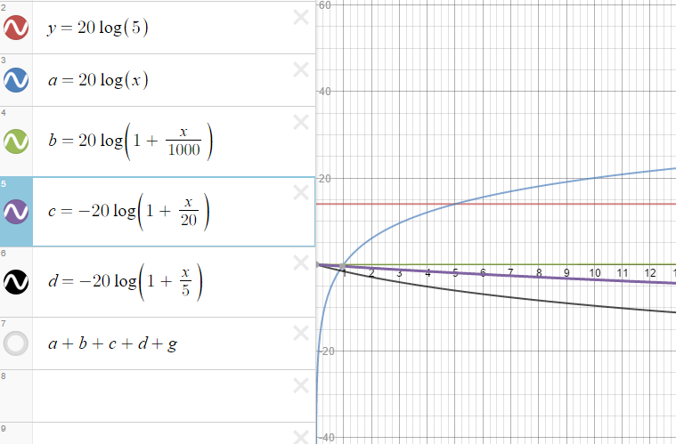
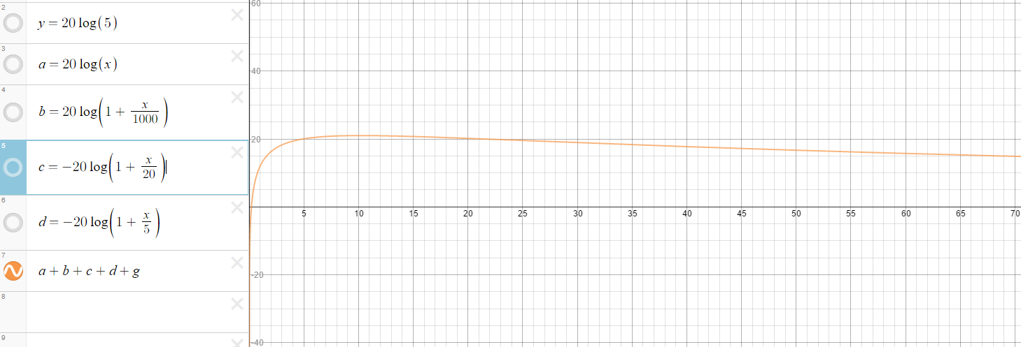
As you should be able to see, the 2nd image is simply all of the functions from the first image added together.
It should be important to note that due to my current software limitations, I could not use the typical Semi-Log graphing style on the x-axis which is typical for Bode plots. This means that this plot is not exact. You can see the actual bode plots for this transfer function with Wolfram Alpha
Phase Plots
Q: So then how can we plot the phase angle with respect to the frequency, \(\omega\)?
If we simply take what we know about complex numbers like above we find that \(a + jb, \theta = arctan\frac{b}{a}\)
Let’s first take a look at the function of \(arctan(\omega)\) to refresh us.
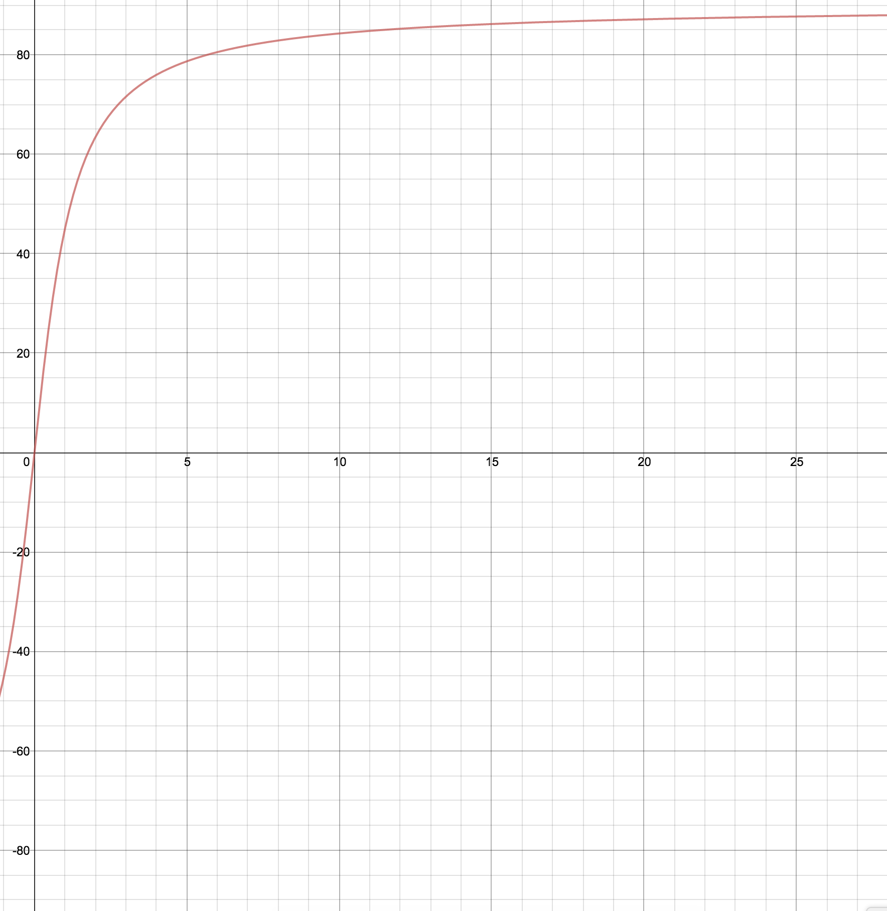
Also recall that \(\lim_{\omega\to\infty} arctan(\omega) = 90^{\circ}\)
So this tells us that the component which is \(arctan(\omega)\) approaches 90 with large values of \(\omega\).
So on a semi log scale we can approximate by saying that for all values \(\omega\), that \(arctan(\omega) = 90\)
This will give us the angle for all of the different components. We can then add the respective phase angles together after plotting.
Recall that \(arctan(1)=45^{\circ}\) as well.
So this means that for approximation of terms which are \(arctan(1 + \frac{2}{\omega_0})\) that at the corner frequency that we will have a value of \(45^{\circ}\). However, that this will be positive or negatively sloping depending on whether the term is in the numerator or denominator of the transfer function.
So then a decade prior to the corner frequency, the value should be \(\approx 0\).
Then a decade after the corner frequency will have a value \(\approx \pm 90\) where the \(\pm\) depends on whether the term is in the numerator or denomitor.
- POSITIVE for the numerator
- NEGATIVE for the denominator
Depending on any constants which might be present in the transfer function typical bode approximations will say that \(arctan(k)\) where \(k\) is a constant, such as our \(arctan(5)\) will be equal to zero, or \(\pm 90^{\circ}\) (depending where the constant lies.
If the constant is on an order of magnitude which is \(> 10^1\) Then it should be plotted on the graph, otherwise it should be approximated as \(\approx 90\)
We then simply add the slopes of all terms together to find the phase
So then to plot our phase diagram from the transfer function:
\[H(s) = \frac{5s(1+\frac{s}{1000})}{(1 + \frac{s}{20})(1 + \frac{s}{5})}\]
We can then take the arctan of each term, and then add their value together.
This gives us the components
- \[arctan(5) \approx 90\]
- \[arctan(1 + \frac{s}{1000})\]
- \[arctan(1 + \frac{s}{20})\]
- \[arctan(1 + \frac{s}{5})\]
From here we simply add the functions to find the phase plot
So now let’s take a look at what the graph will look like (note this is not on a semi-log scale!)
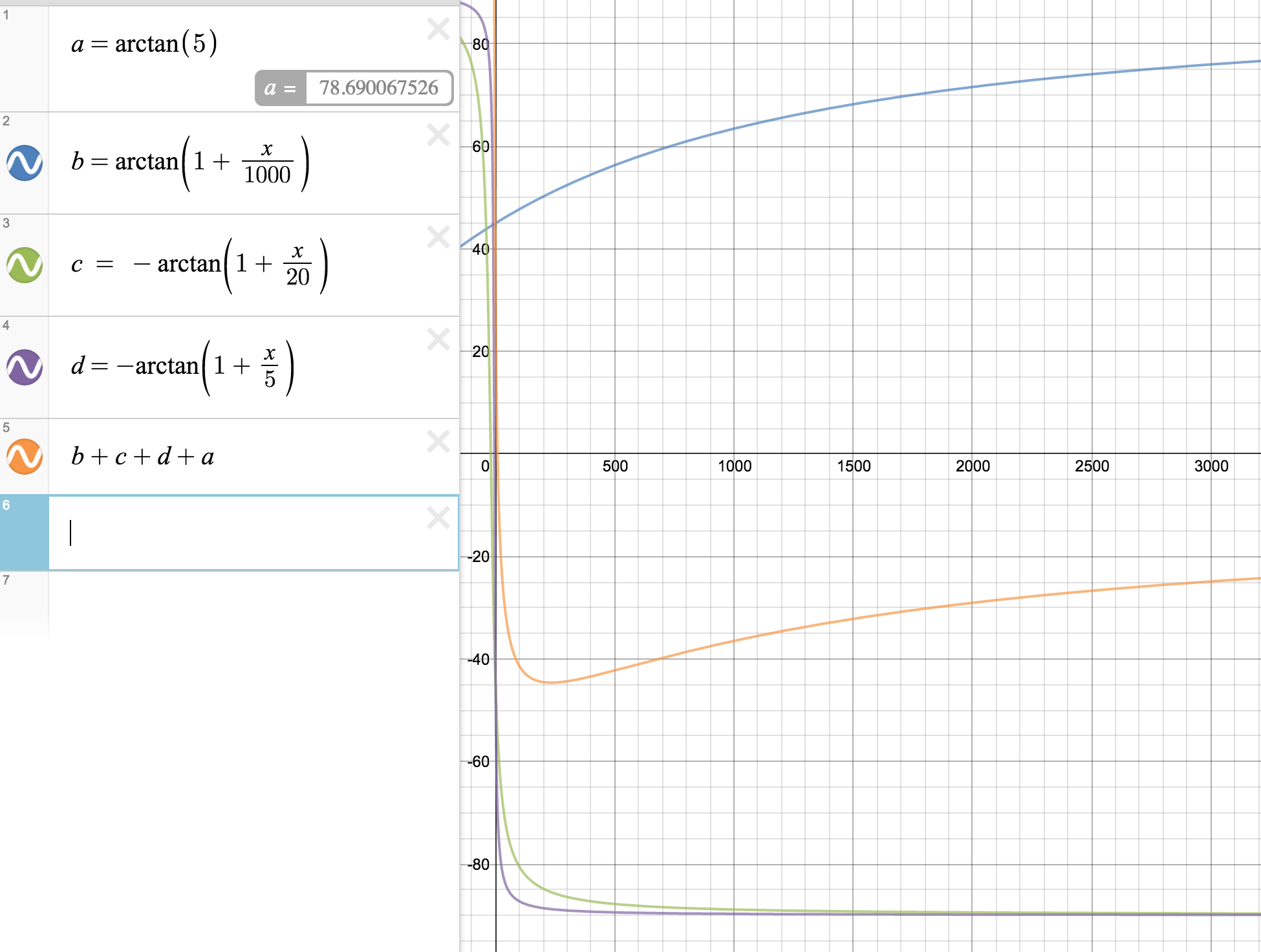
We can see that from this